LAW OF VARIABLE PROPORTIONS
Law of variable proportions occupies an important place in economic theory. This law examines the production function with one factor variable, keeping the quantities of other factors fixed. In other words, it refers to the inputoutput relation when the output is increased by varying the quantity of one input. When the quantity of one factor is varied, keeping the quantity pf the other factors constant, the proportion between the variable factor and the fixed factor is altered; the ratio of employment of the variable factor to that of the fixed factor goes on increasing as the quantity of the variable factor is increased. Since under this law we study the effects on output of variations in factor proportions, this is known as the law of variable proportions. The law of variable proportions is the new name for the famous “Law of Diminishing Returns” of classical economics. This law has played a vital role in the history of economic thought and occupies an equally important place in modern economic theory and has been supported by the empirical evidence about the real world. The law of variable proportions or diminishing returns has been stated by various economists in the following manner :
“As equal increments of one input are added; the inputs of other productive services being held constant, beyond a certain point the resulting increments of product will decrease, i.e. the marginal products will diminish” (G. Stigler).
“As the proportion of one factor in a combination of factors is increased, after a point, first the marginal and then the average product of that factor will diminish.” (F. Benham).
“An increase in some inputs relative to other fixed inputs will, in a given state of technology, cause output to increase; but after a point the extra output resulting from the same additions of extra inputs will become less and less.” (P.A. Samuelson). Marshall discussed the law of diminishing returns in relation to agriculture. He defines the law as follows;
“An increase in the capital and labour applied in the cultivation of land causes in general a less than proportionate increase in the amount of product raised unless it happen to coincide with an improvement the arts of agriculture”.
Assumptions of the Law of Variable Proportions.
The law of variable proportions (or diminishing returns) as stated above holds good under the following conditions :
1. Firstly, the state of technology is assumed to be given and unchanged. If there is improvement in technology, then marginal and average product may rise instead of diminishing.
2. Secondly, there must be some inputs whose quantity is kept fixed. It is only in this way that we can alter the factor proportions and know its effects on output. This law does not apply in case all factors are proportionately varied. Behaviour of output as a result of the variations in all inputs is discussed under “returns to scale”.
3. Thirdly, the law is based upon the possibility of varying the proportions in which the various factors can be combined to produce a product. The law does not apply to those cases where the factors must be used in fixed proportions to yield a product. When the various factors are required to be used in rigidly fixed proportions, then the increase in one factor would not lead to any increase in output, that is, the marginal product of the factor will then be zero and not diminishing
Three Stages of the Law of Variable Proportions
The varying quantity of one factor combined with a fixed quantity of the other can be divided into three distinct stages. In order to understand these three stages it is better to graphically illustrate the production function with one factor variable. This is done in Fig.4. In this figure, on the X-axis is the quantity of the variable factor and on the Y axis are the total, average and the marginal product. How the total product, average product and marginal product of the variable factor change as a result of the increase in its quantity, that is, by increasing the quantity of one factor to a fixed quantity of the others will be seen in Fig. 4. The total pro-duct curve TP goes on increasing to a point and after that it starts declining. Average and marginal product curves also rise and then decline; marginal product curve starts declining earlier than the average product curve. The behaviour of these total, average and marginal products of the variable factor consequent on the increase in its amount is generally divided into three stages which are explained below.
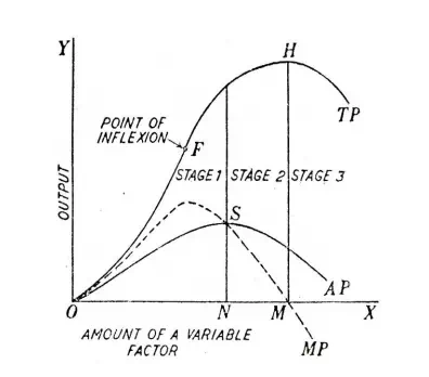
Stage 1 is known as the stage of increasing returns because average product of the variable factor increases throughout this stage. It is notable that the marginal product in this stage increases but in a later part it starts declining but remains greater than the average product so that the average product continues to rise.
Stage 2 : Stage of Diminishing returns. In stage 2, the total product continues to increase at a diminishing rate until it reaches its maximum point H where the second stage ends. In this stage both the marginal product and average product of the variable factor are diminishing but are positive. At the end of the second stage, that is, at point M marginal product of the variable factor is zero (corresponding to the highest point 27 of the total product curve TP) Stage 2 is very crucial and important because the firm will seek to produce in its range. This stage is known as the stage of diminishing returns as both the average and marginal products of the variable factor continuously fall during this stage.
Stage 3 : Stage of Negative Returns. In stage 3 total product declines and therefore the total product curve TP slopes downward. As a result, marginal product of the variable factor is negative and the marginal product curve MP goes below the X-axis. In this stage, variable factor is too much relative to the fixed factor. This stage is called the stage of negative returns, since the marginal product of the variable factor is negative during this stage.