10 advanced formatting tricks for Excel users
Most Excel users know how to apply basic numeric and text formats. But users who push beyond the basics will create more readable and effective sheets. In addition, knowing how to apply just the right formatting to specific cells quickly and easily helps users work more efficiently. These 10 tips will help users get more out of Excel's formatting features.
The fill handle is a versatile and powerful tool. Besides copying formulas and creating series, the fill handle can copy formats with just a few quick clicks:
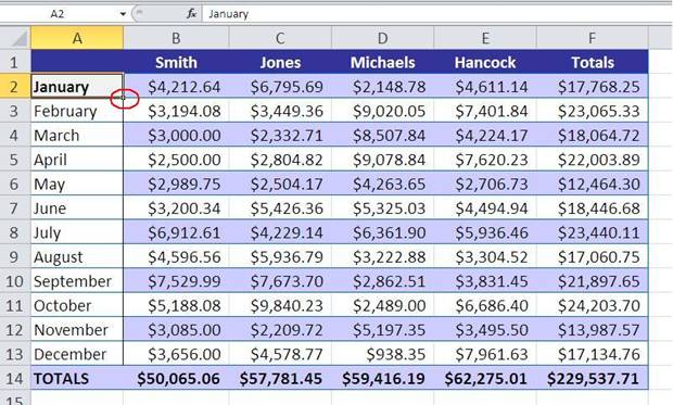
1. Select the cell that contains the formatting you want to copy. In Figure A, I've selected A2 to copy the bold font and gray fill color to the remaining cells in column A.
2. Double-click the cell's fill handle. The fill handle's series behavior has kicked into gear by overwriting the TOTALS label with January. Don't worry about that, you can undo that next.
3. Click the resulting AutoFill Options control to display the list shown in Figure B.
4. Select the Fill Formatting Only option.

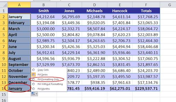
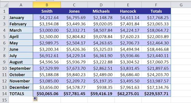
You can see that the fill handle canceled the series values in Figure C. In addition, the action reverted to the original data and applied the formats from A3 to the destination range. This method isn't superior to Format Painter, but you won't have to select the target range, which can be awkward with a large one.
Another quick copy trick utilizes the Paste feature. Again, the Format Painter works great with a small range, but this trick is helpful when copying formats to an entire column or row:
1. Select the source cell and press [Ctrl]+C.
2. Click anywhere inside the destination column or row.
3. Press [Ctrl]+[Spacebar] to select the entire column or [Shift]+[Spacebar] to select the entire row. (This works only with a blank data range.) 2010: With the column or row selected, choose Formatting from the Paste drop-down (in the Clipboard group). 2007: Choose Paste Special from the Paste drop-down and click Formats in the Paste section. 2003: Right-click a selected cell and choose Paste Special from the submenu. In the resulting dialog, click Formats in the Paste section.
4. Using Live Preview, you can see what the applied formats will look like. Click OK if you decide to apply them.
You can also format a new chart using Paste. Select the source chart and press [Ctrl]+C. Select the destination chart and choose Paste Special from the Paste drop-down. Choose Formats and click OK.
If you use the same custom cell styles in multiple workbooks, don't spend time re-creating each style. Instead, copy the style from one file to another as follows:
1. Open the source workbook and a destination workbook.
2. From the destination workbook, click Cell Styles in the Styles group on the Home tab. In Excel 2003, choose Styles from the Format menu.
3. Choose Merge Styles at the bottom of the gallery.
4. In the resulting dialog, select the open workbook that contains the styles you want to copy.
5. Click OK twice.
If you want all new workbooks to share the same custom style, open Excel's default workbook, book.xltx as the destination. (Open book.xlt in Excel 2003.) Add the style, then save and close the template file. All new workbooks based on book.xltx will contain the merged styles.
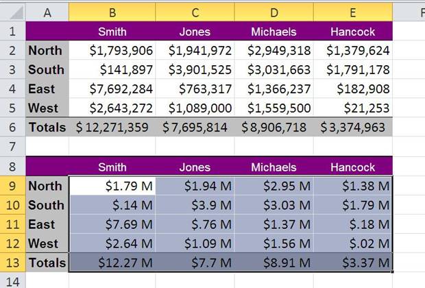
Numbers with a few digits are easy to read. Once you drop in that second thousands separator, numbers become less readable, especially if your data contains lots of them. Fortunately, a custom format can reduce the number of digits, making them easier to read, but without changing the scale. To illustrate, we'll apply this custom format to the values in the bottom range (so you can compare):
1. Select B9:E13 and click the Number group's dialog launcher or press [Ctrl]+1 to display the Format Cells dialog.
2. From the Category list (on the Number tab) choose Custom.
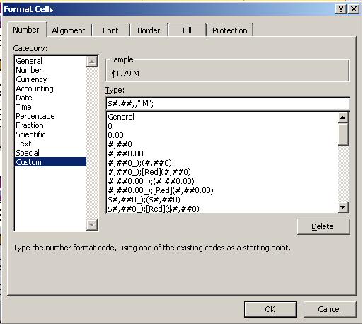
3. In the Type control, enter the $#.##,," M"; format string, as shown in Figure D. The pound sign combined with the two comma characters displays a character in the millions position, if one exists. The M component displays a literal M character, to denote millions.
4. Click OK to see the results in Figure E.
Refer to Create or delete a custom number format for a comprehensive list of formatting codes.
Using a Cell Style to identify purpose helps users acclimate quicker. It also provides an easy way to ensure consistency in an organization. For example, you might use color to distinguish input and label cells. Using a Cell Style is an efficient way to put that convention to work. Let's illustrate this concept by creating a Cell Style for input cells:
1. Click the Home tab and then click Cell Styles in the Styles group. In Excel 2003, choose Style from the Format menu and skip to #3.
2. Click New Cell Style at the bottom of the list.
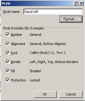
3. In the resulting dialog box, enter a name for the style, such as InputCell.
4. Click Format. In Excel 2003, click Modify.
5. Click the Border tab and choose the Outline option in the Presets section.
6. Click the Fill tab and choose light blue.
7. Click OK to view the selected formats shown in Figure F.
8. Click OK again.
Anytime you want to indicate an input cell or range, do the following:
1. Select the cell.
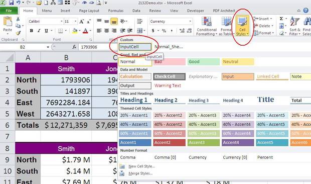
2. On the Home tab, click the Cell Styles option. In Excel 2003, choose Style from the Format menu.
3. Click InputCell as shown in Figure G and Excel will apply that style to the selected cell or range. In Excel 2003, choose InputCell from the drop-down list and click Add.
Using a Cell Style is efficient for the workbook's author, but it also helps users quickly identify a cell or range's purpose.
An efficient copy technique is a good tool, especially if you can choose what to copy on the fly. To do so, select the destination cell or range. Then, right-click the border and drag it to the target cell. When you release the mouse, Excel will display the submenu shown in Figure H. Choose the Copy Here As Formats Only option. That was easy!

Adding a background image to a sheet is so easy that you might be tempted to spruce up all your sheets this way. (You'll refrain from doing so, of course.) To add an image to a sheet's background, do the following:
1. Click the Page Layout tab.
2. Click the Background option in the Page Setup group.
3. Browse to the file and double-click it.
If you select a range and choose a built-in format from the Format As A Table drop-down, Excel (2007 and later) converts the range to a Table object. If the format works for you, but you don't want a Table object, you can keep the format and dump the Table. Doing so takes a few clicks, but probably fewer than formatting manually. To format the data range quickly using a built-in Table format, do the following:
1. Click anywhere inside the data range.
2. On the Home tab, click the Format As Table drop-down and choose a format from the gallery.
3. Choose appropriately when Excel asks if the range has headers and click OK.
4. Click anywhere inside the table.
5. With the contextual Design tab current, choose Convert To Range in the Tools group.
6. Click Yes to confirm the action.
You'll format a data range with only six clicks (or a few more depending on how many times you click the thumb in the gallery).
When you use the Number Formats drop-down in the Number group (on the Home tab), you're actually applying a style -- a style you can control. For instance, the Percent style displays two decimal values, and you might want to inhibit all decimal values for percentages. To do so, click the Number group's dialog launcher, click the Number tab, choose Percentage, change the Decimal Places value to 0, and click OK.
We tend to think of these styles as formats set in stone, but they're not. Modify them to suit your needs. Styles are available only to the workbook in which you save them, but you can modify the styles in your templates.
For a quick one-time solution, you can format some values as you enter them:
· To enter currency, type a dollar sign ($) before typing the value to apply the Currency format.
· To enter most fractions, type 0. Then, press the spacebar and type the fraction, including the slash. Excel will display the value as a fraction and store the decimal value.
· To enter a percentage, simply follow the value with a percent sign.