Vehicle acceleration and maximum speed modeling and simulation

In engineering, simulations play a critical part in the design phase of any system. Through simulation we can understand how a system works, how it behaves under predefined conditions and how the performance is affected by different parameters.

In this article we are going to use a simplified mathematical model of the longitudinal dynamics of a vehicle, in order to evaluate the acceleration performance of the vehicle (0-100 kph time) and determine the maximum speed.

To validate the accuracy of our mathematical model, we are going to compare the simulation result with the advertised parameters of the vehicle.

Input data

The vehicle parameters are taken from a rear-wheel drive (RWD) 16MY Jaguar F-Type:

Engine		3-litre V6 DOHC V6, aluminium-alloy cylinder block and heads
Maximum torque [Nm]		450
Engine speed @ maximum torque [rpm]		3500
Maximum power [HP]		340
Engine speed @ maximum power [rpm]		6500
Transmission type		automatic, ZF8HP, RWD
Gear ratio	1^st	4.71
	2^nd	3.14
	3^rd	2.11
	4^th	1.67
	5^th	1.29
	6^th	1.00
	7^th	0.84
	8^th	0.67
	Final drive (i₀)	3.31
Tire symbol		295/30ZR-20
Vehicle mass (curb) [kg]		1741
Aerodynamic drag, C_d [-]		0.36
Frontal area, A [m²]		2.42
Maximum speed [kph]		260
Acceleration time 0-100 kph [s]		5.3

From data available on the internet, we can also extract the static engine torque values at full load, function of engine speed:

Engine speed points (full load) [rpm]	1000	2020	2990	3500	5000	6500
Engine static torque points (full load) [Nm]	306	385	439	450	450	367

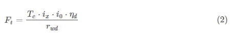
Vehicle layout

The powertrain and drivetrain of a RWD vehicle consists of:

§ engine

§ torque converter (clutch)

§ automatic (manual) transmission

§ propeller shaft

§ differential

§ drive shafts

§ wheels

Image: Vehicle rear-wheel drive (RWD) powertrain diagram

For simplicity, for our simulation example we are going to make the following assumptions:

§ the engine is only a source of torque, without any thermodynamics or inertia modeling

§ the engine is running at full load all the time

§ the effect of the torque converter is not considered

§ the gear shifting is performed instantaneous disregarding any related slip or dynamics

§ the effects of the propeller shaft and drive shafts are not considered

§ the tires have constant radius and the effect of slip is not considered

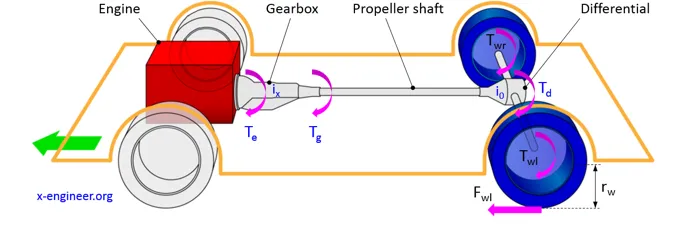
The mathematical model is going to be implemented as a block diagram in Xcos (Scilab), based on the following equations.

Mathematical equations

The vehicle movement is described by the longitudinal forces equation:

where:

F_t [N] – traction force
F_i [N] – inertial force
F_s [N] – road slope force
F_r [N] – road load force
F_a [N] – aerodynamic drag force

The traction force can be regarded a a “positive” force, trying to move the vehicle forward. All the other forces, are resistant, “negative” forces which are opposing motion, trying to slow down the vehicle.

As long as the traction force will be higher than the resistances, the vehicle will accelerate. When the traction force is smaller compared with the sum of resistant forces, the vehicle will decelerate (slow down). When the traction force is equal with the sum of resistant forces, the vehicle will maintain a constant speed.

The traction force [N] depends on the engine torque, engaged transmission gear ratio, final drive ratio (differential) and wheel radius:

where:

T_e [Nm] – engine torque
i_x [-] – transmission gear ratio
i₀ [-] – final drive ratio
η_d [-] – driveline efficiency
r_wd [m] – dynamic wheel radius

The dynamic wheel radius [m] is the radius of the wheel when the vehicle is in motion. It is smaller than the static wheel radius r_ws because the tire is slightly compressed during vehicle motion.

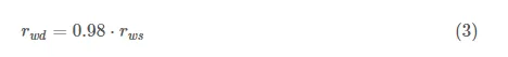
The static wheel radius [m] is calculated based on the tire symbol (295/30ZR-20). For a better understanding of the calculation method read the article How to calculate the wheel radius.

The inertial (resistant) force [N] is given by the equation:

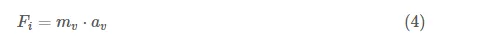
where:

m_v [kg] – total vehicle mass
a_v [m/s²] – vehicle acceleration

The total vehicle mass [kg] consists of the curb vehicle mass, the driver’s mass and an additional mass factor. The mass factor takes into account the effect of the rotating components (crankshaft, gearbox shafts, propeller shaft, drive shafts, etc.) on the overall vehicle inertia.

where:

f_m [-] – mass factor
m_cv [kg] – curb vehicle mass
m_d [m] – driver mass

The road slope (resistant) force [N] is given by the equation:

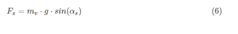
where:

g [m/s²] – gravitational acceleration
α_s [rad] – road slope angle

The road load (resistant) force [N] is given by the equation:

where:

c_r [-] – road load coefficient

The aerodynamic drag (resistant) force [N] is given by the equation:

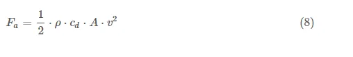
where:

ρ [kg/m³] – air density at 20 °C
c_d [-] – air drag coefficient
A [m²] – vehicle frontal area
v [m/s] – vehicle speed

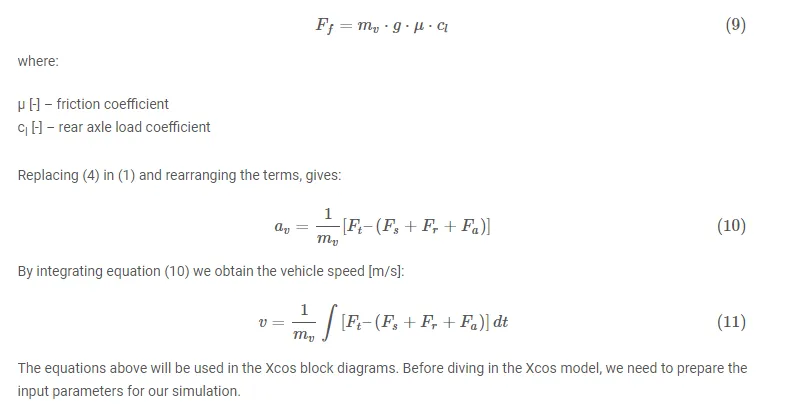
The traction force is limited by the wheel friction coefficient in the contact patch. The maximum friction force [N] that allows traction is: