Curve Interpolation Methods and Options

The RMC supports several interpolation methods and options to satisfy a wide range of curve applications.

Interpolation Methods

The interpolation method is specified in the Properties pane in the Curve tool, or in the Curve Add (82) command. Choose from one of the methods below. The Cubic (2) method is the most common method and creates the smoothest motion.

·         Cubic (2)

The curve will smoothly go through all points. This is the most common interpolation method. This method will create smooth motion.

On position axes, the Velocity Feed Forward and Acceleration Feed Forward will apply to cubic interpolated curves, but higher order gains should not be used, such as the Jerk Feed Forward, Double Differential Gain, and Triple Differential Gain.

On pressure or force axes, the Pressure/Force Rate Feed Forward will apply.

·         Linear (1)

The curve will consist of straight-line segments between each point. Because the velocity is not continuous, a position axis will tend to overshoot at each point. This type of curve is typically more suitable for pressure or force axes.

On position axes, the Target Acceleration will always be zero. Therefore, the Acceleration Feed Forward will have no effect for linear interpolated curves.

·         Constant (0)

The curve will consist of step jumps to each point. The curve will not be continuous. This method is seldom used, but may be useful in applications where step jumps are desired, such as some blow-molding systems. This method requires that the axis not be tuned very tightly, or the axis may oscillate and Output Saturated errors may occur. The Position I-PD control algorithm is recommended for following constant interpolated curves.

On position axes, the Target Velocity and Target Acceleration will always be zero. Therefore, the Velocity Feed Forward and Acceleration Feed Forward will have no effect for constant interpolated curves.

On pressure or force axes, the Target Rate will always be zero. Therefore, the Pressure/Force Rate Feed Forward will have no effect for constant interpolated curves.

Interpolation Options

The interpolation options are specified in the curve data. The available options depend on the interpolation method, as shown in the table below. Add the numbers for each desired option. For example, to choose Cyclic Curve and Overshoot Protection, the Interpolation Option value would be 2+8 = 10.

Endpoint Behavior

This option defines the behavior at the endpoints. Each option below shows a plot for the following cubic curve data with 9 points at 0.25 second intervals:

·         +0 Zero-Velocity Endpoints

The endpoints will have zero velocity and acceleration. This is the most commonly-used option. Curves with zero-velocity endpoints can be repeated cyclically.

·         +1 Natural-Velocity Endpoints

The endpoints will have their velocity automatically selected to match the natural slope of the curve at the endpoints. The acceleration at the endpoints will be zero. Curves with natural-velocity endpoints cannot be repeated cyclically because the endpoint velocities are typically not equal.

·         +2 Cyclic Curve

The endpoints are assumed to wrap. Therefore the acceleration, velocity, and position will be continuous between cycles of this curve, although the velocity and acceleration at each endpoint will not necessarily be zero.

If the y-values of the first and last points are not equal, and the curve is run for more than 1 consecutive cycle, the curve will be automatically offset so that the first point of the next cycle matches the last point of the previous cycle.

For Advanced format curves, if an endpoint is defined as a Fixed Velocity type, it will use that velocity even if the curve is cyclic. Setting each endpoint to a different fixed velocity will cause a discontinuity in the velocity between cycles of the curve, but the curve can still be used cyclically.

Overshoot Protection

The Overshoot Protection option prevents the curve from exceeding a local maximum or local minimum point. A local maximum occurs where a point is greater than or equal to both the preceding point and the following point. A local minimum occurs where a point is less than or equal to both the preceding point and the following point. Overshoot protection will not prevent overshooting in other locations.

When overshoot protection is enabled, the velocity is set to zero at each local minimum/maximum point, which eliminates the chance of the curve overshooting that point for the curve segments on either side of the point.

For Advanced format curves, Overshoot Protection will not apply to Fixed-Velocity points, or points at the beginning or end of a Constant-Velocity segment.

Example 1

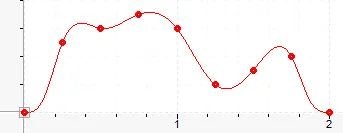
Consider the cubic curve data in the Endpoint Behavior section above. Without Overshoot Protection enabled, the curve looks like this:

Notice that the curve overshoots the points after times 0.75, 1.25, and before 1.75.

With overshoot protection enabled, the curve will look like this:

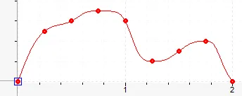
Notice that the curve no longer overshoots the points after times 0.75, 1.25, and before 1.75. Notice, however, that the curve still overshoots between points 0.25 and 0.5 because neither point is a local minimum or maximum.

Auto-Constant Velocity

The Auto-Constant Velocity option will automatically insert a linear segment in the curve if three or more data points are in a straight line.

If you have also selected Overshoot Protection, be aware that the points identified as local minimums or maximums do not count as consecutive points for the Auto-Constant Velocity (see the example below).

For Advanced format curves, be aware that the Fixed Velocity type points do not count as consecutive points for the Auto-Constant Velocity (see the example below).

Example 2

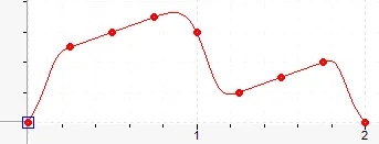
Consider the cubic curve data in the Endpoint Behavior section above. The points at times 0.25, 0.50, and 0.75 are in a straight line, as are the points at times 1.25, 1.50, and 1.75. With the Auto-Constant Velocity option, the curve will look like this:

Example 3

Consider this same curve with both Overshoot Protection and Auto-Constant Velocity enabled. This particular curve ends up looking the same as it does with only Overshoot Protection, because both constant-velocity segments are lost because at least one of each set of 3 consecutive points was identified by Overshoot Protection as a local minimum or maximum.