Geometric Probability
Geometric probability is a tool to deal with the problem of infinite outcomes by measuring the number of outcomes geometrically, in terms of length, area, or volume. In basic probability, we usually encounter problems that are "discrete" (e.g. the outcome of a dice roll; see probability by outcomes for more). However, some of the most interesting problems involve "continuous" variables (e.g., the arrival time of your bus).
Dealing with continuous variables can be tricky, but geometric probability provides a useful approach by allowing us to transform probability problems into geometry problems. If this sounds surprising, take a look at the following problem:
Intuitively, the answer seems to be \frac{1} {2}21. We can show this geometrically by considering a point chosen randomly on a 1-dimensional number line: the length of the number line between 12:30 pm and 1 pm is equal to the length from 12 pm to 12:30 pm.
While this example is fairly straightforward, many complicated problems can be solved simply by using geometric probability. On this page, we will start with 1D examples, which are the simplest and easy to understand and then work our way up to 2D, 3D, and higher dimensions.
1-dimensional Geometric Probability
Let's look more at the situation where XX is a random real number, as mentioned in the Introduction section. To reiterate, the core idea in one-dimensional (1D) geometric probability is translating a probability question into a geometry problem on a number line, where we measure outcomes with length. To make sure you've got this concept down, try this problem related to rounding errors:
The reason as to why this works is a more advanced topic, which deals with the idea of measure theory. Measure theory gives a rigorous framework for probability theory, including probabilities on finite sets. Measure theory is also the key idea behind integration in calculus, and can be used to find integrals of functions that seem non-integrable using “standard” methods. These two ideas are not unrelated, as at a fundamental level, probability theory is just a special case of integration.
We will do a few more examples on working with geometric probabilities in higher dimensions to get a better feel for how to work with the concept. It is often helpful to use a figure to help with understanding and solving these types of problems
2-dimensional Geometric Probability
The difficulty associated with geometric probability usually comes from one of two areas: the first is finding a good way to model the problem geometrically, and the second is in trying to determine the areas/volumes of particular regions in order to calculate the relative probabilities. As in finite probability, it is sometimes simpler to find the probability of the complement.
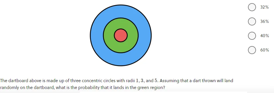
To make sure you've got down the basic ideas of 2D geometric probability, try this similar question. Note that many 2D geometry problems, such as the one below, use the ideas of composite figures. If you are not familiar with that concept, you may want to take a look at composite figures first.
However, one of the most powerful uses of geometric probability is applying it to problems that are not inherently geometric. Identifying when and how to use geometric probability is never obvious, but a good sign is that you are dealing with probabilities in a situation with continuous variables.
3-dimensional Geometric Probability
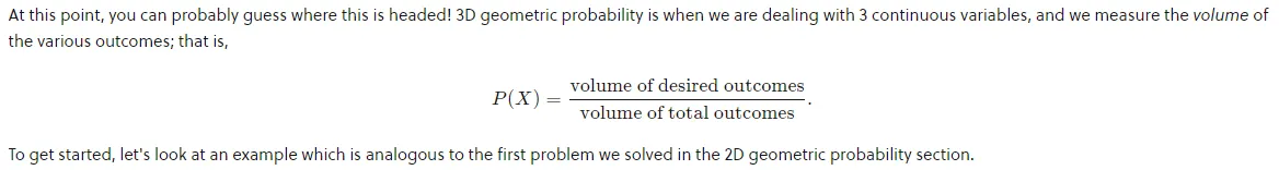
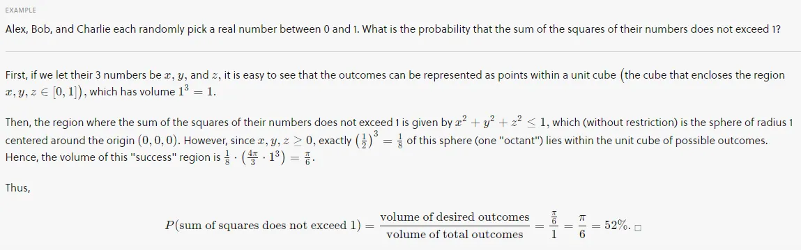
Of course, not all problems will be so explicitly geometric in nature. As usual, one of the signs that we might want to apply geometric probability is that we are dealing with continuous variables. Let's see how we can approach the following example: