The Primal and Dual Linear Programming Problems
Linear programming problems come in pairs — a primal linear program (P) and an associated dual linear program (D). The linear objective function and the linear constraints of primal and dual programs of the linear programming problem are related in a specific way. I illustrate the mathematical statement of a linear programming problem with the following example.
Primal Linear Program | Dual Linear Program |
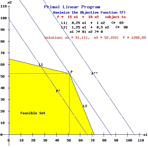
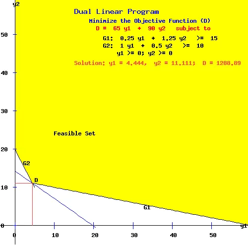
The following diagrams help one to visualize the primal and dual problems and suggest a way of solving linear programming problems. The area in yellow, called the feasible set, represents values of x1 and x2, (or y1 and y2), that satisfy the constraints L1 and L2, (or G1 and G2). Such vectors x = (x1, x2) (or y = (y1, y2) are called feasible vectors for the primal program (or dual program).
The lines P', P, and P'' in the primal diagram represent the objective function for different values of P, (988.89, 1288.89, 1588.89). Where P = 1288.89, the objective function (P) intersects the feasible set only at the point (x1, x2) = (51.111, 52.222). Here P attains its maximum value on the feasible set.

The points (0,0 ), (72, 0), (51.111, 52.222), and (0, 65) are called the vertices of the feasible set. An optimal program obtains at a vertex of the feasible set.
Similarly, in the dual diagram where D = 1288.89, the objective function (D) intersects the feasible set only at the point (y1, y2) = (4.444, 11.111). Here D attains its minimum on the feasible set.

Notes:
1. In the primal problem, the vector (x1, x2) = (51.111, 52.222) is the optimal primal program. For any other point in the feasible set, like (x'1, x'2) = (40, 40), the value of the objective function is less than the value of the objective function at the optimal program. i.e.,
15 x'1 + 10 x'2 = 15*40 + 10*40 = 1000 < 1288.89 = 15*51.111 + 10*52.222 = P
2. In the dual problem, the vector (y1, y2) = (4.444, 11.111) is the optimal dual program. For any other point in the feasible set, like (y'1, y'2) = (20, 20), the value of the objective function is greater than the value of the objective function at the optimal program. i.e.,
D = 1288.89 = 65(4.444) + 90(11.111) < 3100 = 65(20) + 90(20) = 65 y'1 + 90 y'2
This is known as Economical Equilibrium.