Object Detection
An approach to building an object detection is to first build a classifier that can classify closely cropped images of an object. Fig 2. shows an example of such a model, where a model is trained on a dataset of closely cropped images of a car and the model predicts the probability of an image being a car.
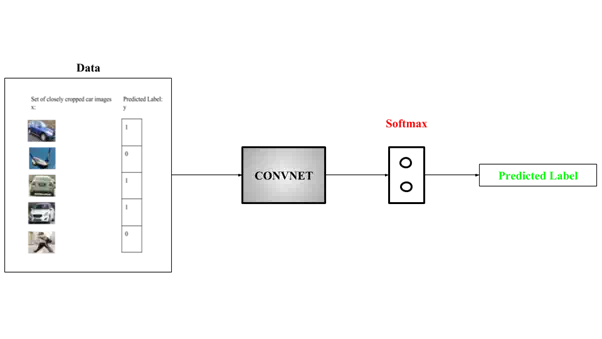
Fig 2. Image classification of cars
Now, we can use this model to detect cars using a sliding window mechanism. In a sliding window mechanism, we use a sliding window (similar to the one used in convolutional networks) and crop a part of the image in each slide. The size of the crop is the same as the size of the sliding window. Each cropped image is then passed to a ConvNet model (similar to the one shown in Fig 2.), which in turn predicts the probability of the cropped image is a car.

Fig 3. Sliding windows mechanism
After running the sliding window through the whole image, we resize the sliding window and run it again over the image again. We repeat this process multiple times. Since we crop through a number of images and pass it through the ConvNet, this approach is both computationally expensive and time-consuming, making the whole process really slow. Convolutional implementation of the sliding window helps resolve this problem.
Convolutional implementation of sliding windows
Before we discuss the implementation of the sliding window using convents, let’s analyze how we can convert the fully connected layers of the network into convolutional layers. Fig. 4 shows a simple convolutional network with two fully connected layers each of shape (400, ).
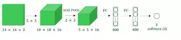
Fig 4. Sliding windows mechanism
A fully connected layer can be converted to a convolutional layer with the help of a 1D convolutional layer. The width and height of this layer are equal to one and the number of filters are equal to the shape of the fully connected layer. An example of this is shown in Fig 5.
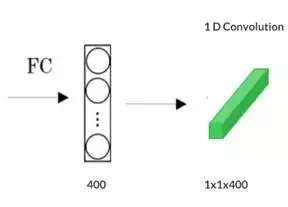
Fig 5. Converting a fully connected layer into a convolutional layer
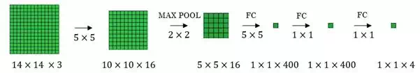
We can apply this concept of conversion of a fully connected layer into a convolutional layer to the model by replacing the fully connected layer with a 1-D convolutional layer. The number of the filters of the 1D convolutional layer is equal to the shape of the fully connected layer. This representation is shown in Fig 6. Also, the output softmax layer is also a convolutional layer of shape (1, 1, 4), where 4 is the number of classes to predict.
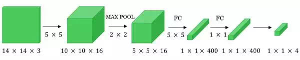
Fig 6. Convolutional representation of fully connected layers.
Now, let’s extend the above approach to implement a convolutional version of sliding window. First, let’s consider the ConvNet that we have trained to be in the following representation (no fully connected layers).
Let’s assume the size of the input image to be 16 × 16 × 3. If we’re to use a sliding window approach, then we would have passed this image to the above ConvNet four times, where each time the sliding window crops a part of the input image of size 14 × 14 × 3 and pass it through the ConvNet. But instead of this, we feed the full image (with shape 16 × 16 × 3) directly into the trained ConvNet (see Fig. 7). This results in an output matrix of shape 2 × 2 × 4. Each cell in the output matrix represents the result of a possible crop and the classified value of the cropped image. For example, the left cell of the output (the green one) in Fig. 7 represents the result of the first sliding window. The other cells represent the results of the remaining sliding window operations.
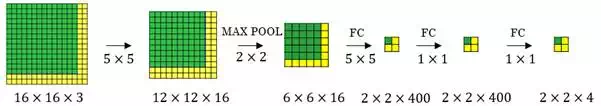
Fig 7. Convolutional implementation of the sliding window
Note that the stride of the sliding window is decided by the number of filters used in the Max Pool layer. In the example above, the Max Pool layer has two filters, and as a result, the sliding window moves with a stride of two resulting in four possible outputs. The main advantage of using this technique is that the sliding window runs and computes all values simultaneously. Consequently, this technique is really fast. Although a weakness of this technique is that the position of the bounding boxes is not very accurate.