Introduction to Object Detection

Humans can easily detect and identify objects present in an image. The human visual system is fast and accurate and can perform complex tasks like identifying multiple objects and detect obstacles with little conscious thought. With the availability of large amounts of data, faster GPUs, and better algorithms, we can now easily train computers to detect and classify multiple objects within an image with high accuracy. In this blog, we will explore terms such as object detection, object localization, loss function for object detection and localization, and finally explore an object detection algorithm known as “You only look once” (YOLO).

Object Localization

An image classification or image recognition model simply detect the probability of an object in an image. In contrast to this, object localization refers to identifying the location of an object in the image. An object localization algorithm will output the coordinates of the location of an object with respect to the image. In computer vision, the most popular way to localize an object in an image is to represent its location with the help of bounding boxes. Fig. 1 shows an example of a bounding box.

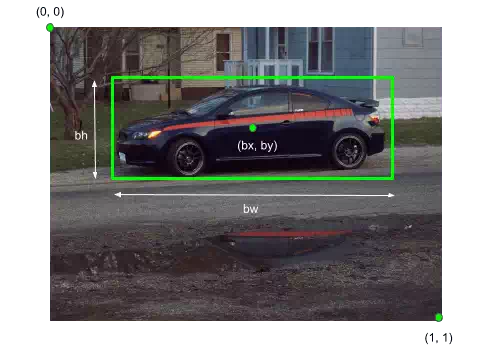
Fig 1. Bounding box representation used for object localization

A bounding box can be initialized using the following parameters:

· bx, by : coordinates of the center of the bounding box

· bw : width of the bounding box w.r.t the image width

· bh : height of the bounding box w.r.t the image height

Defining the target variable

The target variable for a multi-class image classification problem is defined as:

y^=ci

where,
ci = Probability of the ith class.
For example, if there are four classes, the target variable is defined as

y=⎡⎣⎢⎢⎢c1c2c3c4⎤⎦⎥⎥⎥(1)

We can extend this approach to define the target variable for object localization. The target variable is defined as

y=⎡⎣⎢⎢⎢⎢⎢⎢⎢⎢⎢⎢⎢⎢⎢⎢⎢⎢pcbxbybhbwc1c2c3c4⎤⎦⎥⎥⎥⎥⎥⎥⎥⎥⎥⎥⎥⎥⎥⎥⎥⎥(2)

where,
pc = Probability/confidence of an object (i.e the four classes) being present in the bounding box.
bx,by,bh,bw = Bounding box coordinates.
ci = Probability of the ith class the object belongs to.

For example, the four classes be ‘truck’, ‘car’, ‘bike’, ‘pedestrian’ and their probabilities are represented as  c1,c2,c3,c4.  So,

pc={1, ci:{c1,c2,c3,c4}0, otherwise(3)

Loss Function

Let the values of the target variable y are represented as y1, y2, …, y9.

y=[pcbxbybhbwc1c2c3c4]Ty1y2y3y4y5y6y7y8y9(4)

The loss function for object localization will be defined as

L(y^,y)={(y1^–y1)2+(y8^–y8)2+…+(y9^–y9)2(y1^–y1)2,y1=1,y1=0(5)

In practice, we can use a log function considering the softmax output in case of the predicted classes (c1,c2,c3,c4). While for the bounding box coordinates, we can use something like a squared error and for pc(confidence of object) we can use logistic regression loss.

Since we have defined both the target variable and the loss function, we can now use neural networks to both classify and localize objects.