Matching techniques:

Matching is the process of comparing two or more structures to discover their likenesses or differences. The structures may represent a wide range of objects including physical entities, words or phrases in some language, complete classes of things, general concepts, relations between complex entities, and the like. The representations will be given in one or more of the formalisms like FOPL, networks, or some other scheme, and matching will involve comparing the component parts of such structures.

Matching is used in a variety of programs for different reasons. It may serve to control the sequence of operations, to identify or classify objects, to determine the best of a number of different alternatives, or to retrieve items from a database. It is an essential operation such diverse programs as speech recognition, natural language understanding, vision, learning, automated reasoning, planning, automatic programming, and expert systems, as well as many others. In its simplest form, matching is just the process of comparing two structures or patterns for equality. The match fails if the patterns differ in any aspect. For example, a match between the two character strings acdebfba and acdebeba fails on an exact match since the strings differ in the sixth character positions. In more complex cases the matching process may permit transformations in the patterns in order to achieve an equality match. The transformation may be a simple change of some variables to constants, or ti may amount to ignoring some components during the match operation. For example, a pattern matching variable such as ?x may be used to permit successful matching between the two patterns (a b (c d ) e) and (a b ?x e) by binding ?x to (c, d). Such matching are usually restricted in some way, however, as is the case with the unification of two classes where only consistent bindings are permitted. Thus, two patterns such as ( a b (c d) e f) and (a b ?x e ?x) would not match since ?x could not be bound to two different constants.

In some extreme cases, a complete change of representational form may be required in either one or both structures before a match can be attempted. This will be the case, for example, when one visual object is represented as a vector of pixel gray levels and objects to be matched are represented as descriptions in predicate logic or some other high level statements. A direct comparison is impossible unless one form has been transformed into the other. In subsequent chapters we will see examples of many problems where exact matches are inappropriate, and some form of partial matching is more meaningful. Typically in such cases, one is interested in finding a best match between pairs of structures. This will be the case in object classification problems, for example, when object descriptions are subject to corruption by noise or distortion. In such cases, a measure of the degree of match may also be required.

Other types of partial matching may require finding a match between certain key elements while ignoring all other elements in the pattern. For example, a human language input unit should be flexible enough to recognize any of the following three statements as expressing a choice of preference for the low-calorie food item

· I prefer the low-calorie choice.

· I want the low-calorie item

· The low-calorie one please.

Recognition of the intended request can be achieved by matching against key words in a template containing “low-calorie” and ignoring other words except, perhaps, negative modifiers.  Finally, some problems may obviate the need for a form of fuzzy matching where an entity’s degree of membership in one or more classes is appropriate. Some classification problems will apply here if the boundaries between the classes are not distinct, and an object may belong to more than one class.

 Fig 8.1 illustrates the general match process where an input description is being compared with other descriptions. As stressed earlier, their term object is used here in a

general sense. It does not necessarily imply physical objects. All objects will be represented in some formalism such a s a vector of attribute values, prepositional logic or FOPL statements, rules, frame-like structures, or other scheme. Transformations, if required, may involve simple instantiations or unifications among clauses or more complex operations such as transforming a two-dimensional scene to a description in some formal language. Once the descriptions have been transformed into the same schema, the matching process is performed element-by-element using a relational or other test (like equality or ranking). The test results may then be combined in some way to provide an overall measure of similarity. The choice of measure will depend on the match criteria and representation scheme employed.  The output of the matcher is a description of the match. It may be a simple yes or no response or a list of variable bindings, or as complicated as a detailed annotation of the similarities and differences between the matched objects.

`To summarize then, matching may be exact, used with or without pattern variables, partial, or fuzzy, and any matching algorithm will be based on such factors as

· Choice of representation scheme for the objects being matched,

· Criteria for matching (exact, partial, fuzzy, and so on),

· Choice of measure required to perform the match in accordance with the

· chosen criteria, and

· Type of match description required for output.

In the remainder of this chapter we examine various types of matching problems and their related algorithms. We bin with a description of representation structures and measures commonly found in matching problems. We next look at various matching techniques based on exact, partial, and fuzzy approaches. We conclude the chapter with an example of an efficient match algorithm used in some rule-based expert systems.

Typical Matching Process

Structures used in Matching

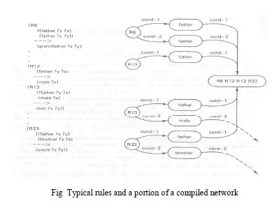
· The types of list structures represent clauses in propositional or predicate logic such as (or ~(MARRIED ?x ?y) ~(DAUGHTER ?z ?y) (MOTHER ?y ?z)) or rules such

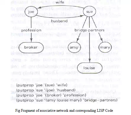
as (and ((cloudy-sky) (low-bar-pressure) (high-humidity)) (conclude (rain likely)) or fragments of associative networks in below Fig

· The other common structures include strings of characters a1 a2 . . . ak , where the ai belong to given alphabet A, vector X = (x1 x2 . . . xn), where the xi represents attribute values, matrices M (rows of vectors), general graphs, trees and sets

Variables

· The structures are constructed from basic atomic elements, numbers and characters

· Character string elements may represent either constants or variables

· If variables, they may be classified by either the type of match permitted or their value domains

· An open variable can be replaced by a single item

· Segment variable can be replaced by zero or more items

· Open variable are replaced with a preceding question mark (?x. ?y, ?class)

· They may match or assume the value of any single string element or word, but they are subject to consistency constraints

· For example, to be consistent, the variable ?x can be bound only to the same top level element in any single structure

· Thus (a ?x d ?x e) may match (a b d b e), but not (a b d a e)

· Segment variable types will be preceded with an asterisk (*x, *z, *words)

· This type of variable can match an arbitrary number or segment of contiguous atomic elements

· For example, (* x d (e g) *y) will match the patterns (a (b c) d (e f) g h), (d (e f ) (g))

· Subject variable may also be subject to consistency constraints similar to open Variables Nominal variables

· Qualitative variables whose values or states have no order nor rank

· It is possible to distinguish between equality or inequality between two objects

· Each state can be given a numerical code

· For example, “marital status” has states of married, single, divorced or  widowed. These states could be assigned numerical codes,

such as married = 1, single = 2, divorced = 3 and widowed = 4

Ordinal variables

· Qualitative variables whose states can be arranged in a rank order

· It may be assigned numerical values

· Foe example, the states very tall, tall, medium, short and very short can be arranged in order from tallest to shortest and can be assigned an arbitrary scale of 5 to 1

Binary variable

· Qualitative discrete variables which may assume only one of two values, such as 0 or 1, good or bad, yes or no, high or low

Interval variables or Metric variables

· Qualitative variables which take on numeric values and for which equal differences between values have the same significance

· For example, real numbers corresponding to temperature or integers corresponding to an amount of money are considered as interval variables

Graphs and Trees

· A graph is a collection of points called vertices, some of which are connected by line segments called edges

· Graphs are used to model a wide variety of real-life applications, including transportation and communication networks, project scheduling, and games

· A graph G = (V, E) is an ordered pair of sets V and E. the elements V are nodes or vertices and the elements of E are a subset of V X V called edges

· An edge joints two distinct vertices in V

· Directed graphs or digraphs, have directed edges or arcs with arrows

· If an arc is directed from node ni to nj , node ni is said to be a parent or successor of nj and nj is the child or successor of ni

· Undirected graphs have simple edges without arrows connecting the nodes

· A path is a sequence of edges connecting two modes where the endpoint of one edge is the start of its successor

· A cycle is a path in which the two end points coincide

· A Connected graph is a graph for which every pair of vertices is joined by a path

· A graph is complete if every element of V X V is an edge

· A tree is a connected graph in which there are no cycles and each node has at most one parent below

· A node with no parent is called root node

· A node with no children is called leaf node

· The depth of the root node is defined as zero

· The depth of any other node is defined to be the depth of its parent plus 1

Sets and Bags

· A set is represented as an unordered list of unique elements such as the set (a d f c) or (red blue green yellow)

· A bag is a set which may contain more than one copy of the same member a,b, d and e

· Sets and bags are structures used in matching operations

Measure for Matching

· The problem of comparing structures without the use of pattern matching variables. This requires consideration of measures used to determine the likeness or similarity between two or more structures

· The similarity between two structures is a measure of the degree of association or likeness between the object’s attributes and other characteristics parts.

· If the describing variables are quantitative, a distance metric is used to measure the proximity

· Distance Metrics

· For all elements x, y, z of the set E, the function d is metric if and only if

            d(x, x) = 0

            d(x,y) ≥ 0

            d(x,y) = d(y,x)

           d(x,y) ≤ d(x,z) + d(z,y)

· The Minkowski metric is a general distance measure satisfying the above assumptions

· It is given by

               N dp = [ Σ|xi - yi|p ]1/p i = 1

· For the case p = 2, this metric is the familiar Euclidian distance. Where p = 1, dp is the so-called absolute or city block distance

· Probabilistic measures

· The representation variables should be treated as random variables

· Then one requires a measure of the distance between the variates, their distributions, or between a variable and distribution

· One such measure is the Mahalanobis distance which gives a measure of the separation between two distributions

· Given the random vectors X and Y let C be their covariance matrix

· Then the Mahalanobis distance is given by D = X’C-1Y

· Where the prime (‘) denotes transpose (row vector) and C-1 is the inverse of C

· The X and Y vectors may be adjusted for zero means bt first substracting the vector means ux and uy

· Another popular probability measure is the product moment correlation r, given by Cov(X, Y) r = -------------------- [ Var(X)* Var(Y)]1/2

· Where Cov and Var denote covariance and variance respectively

· The correlation r, which ranges between -1 and +1, is a measure of similarity frequently used in vision applications

· Other probabilistic measures used in AI applications are based on the scatter of attribute values

· These measures are related to the degree of clustering among the objects

· Conditional probabilities are sometimes used

· For example, they may be used to measure the likelihood that a given X is a member of class Ci , P(Ci| X), the conditional probability of Ci given an observed X

· These measures can establish the proximity of two or more objects Qualitative measures

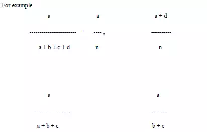
· Measures between binary variables are best described using contingency tables in the below

· Table

· The table entries there give the number of objects having attribute X or Y with corresponding value of 1 or 0

· For example, if the objects are animals might be horned and Y might be long tailed. In this case, the entry a is the number of animals having both horns and

long tails

· Note that n = a + b + c + d, the total number of objects

· Various measures of association for such binary variables have been defined

· Contingency tables are useful for describing other qualitative variables, both ordinal and nominal. Since the methods are similar to those for binary variables

· Whatever the variable types used in a measure, they should all be properly scaled to prevent variables having large values from negating the effects of smaller

valued variables

· This could happen when one variable is scaled in millimeters and another variable in meters

Similarity measures

· Measures of dissimilarity like distance, should decrease as objects become more a like

· The similarities are not in general symmetric

· Any similarity measure between a subject description A and its referent B,denoted by s(A,B), is not necessarily equal

· In general, s(A,B) ≠ s(B,A) or “A is like B” may not be the same as “B is like A”

· Tests on subjects have shown that in similarity comparisons, the focus of attention is on the subject and, therefore, subject features are given higher weights than the

           referent

· For example, in tests comparing countries, statements like “North Korea is similar to Red China” and “Red China is similar to North Korea” were not rated as

symmetrical or equal

· Similarities may depend strongly on the context in which the comparisons are made

· An interesting family of similarity measures which takes into account such factors as asymmetry and has some intuitive appeal has recently been proposed

· Let O ={o1, o2, . . . } be the universe of objects of interest

· Let Ai be the set of attributes used to represent oi

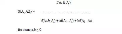
· A similarity measure s which is a function of three disjoint sets of attributes common to any two objects Ai and Aj is given as s(Ai, Aj) = F(Ai & Aj, Ai - Aj, Aj - Ai)

· Where Ai & Aj is the set of features common to both oi and oj

· Where Ai - Aj is the set of features belonging to oi and not oj

· Where Aj - Ai is the set of features belonging to oj and not oi

· The function F is a real valued nonnegative function s(Ai, Aj) = af(Ai & Aj) – bf(Ai - Aj) – cf(Aj - Ai) for some a,b,c ≥ 0

· Where f is an additive interval metric function

· The function f(A) may be chosen as any nonnegative function of the set A, like the number of attributes in A or the average distance between points in A

· When the representations are graph structures, a similarity measure based on the cost of transforming one graph into the other may be used

· For example, a procedure to find a measure of similarity between two labeled graphs decomposes the graphs into basic subgraphs and computes the minimum

cost to transform either graph into the other one, subpart-by-subpart

Matching like Patterns

· We consider procedures which amount to performing a complete match between two structures

· The match will be accomplished by comparing the two structures and testing for equality among the corresponding parts

· Pattern variables will be used for instantiations of some parts subject to restrictions

· Matching Substrings

· A basic function required in many match algorithms is to determine if a substring S2 consisting of m characters occurs somewhere in a string S1 of n characters,

 m ≤ n

· A direct approach to this problem is to compare the two strings character-bycharacter, starting with the first characters of both S1 and S2

· If any two characters disagree, the process is repeated, starting with the second character of S1 and matching again against S2 character-by-character until a match

              is found or disagreements occurs again

· This process continues until a match occurs or S1 has no more characters

· Let i and j be position indices for string S1 and a k position index for S2

· We can perform the substring match with the following algorithm

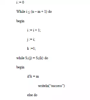
· This algorithm requires m(n - m) comparisons in the worst case

· A more efficient algorithm will not repeat the same comparisons over and over again

· One such algorithm uses two indices I and j, where I indexes the character positions in S1 and j is set to a “match state” value ranging from 0 to m

· The state 0 corresponds to no matched characters between the strings, while state 1 corresponds to the first letter in S2 matching character i in S2

· State 2 corresponds to the first two consecutive letters in S2 matching letters i and i+1 in S1 respectively, and so on, with state m corresponding to a successful match

· Whenever consecutive letters fail to match, the state index is reduced accordingly

Matching Graphs

· Two graphs G1 and G2 match if they have the same labeled nodes and same labeled arcs and all node-to-node arcs are the same

· If G2 with m nodes is a subgraph of G1 with n nodes, where n ≥ m

· In a worst cas match, this will require n!/(n - m)! node comparison and O(m2) arc comparisons

· Finding subgraph isomorphisms is also an important matching problem

· An isomorphism between the graphs G1 and G2 with vertices V1, V2 and edges E1, E2, that is, (V1, E1) and (V2, E2) respectively, is a one-to-one mapping to f between V1 and V2, such that for all v1 € V1, f(v1) = v2, and for each arc e1 € E1 connecting v1 and v1’ , there is a corresponding arc e2 € E2 connecting f(v1) and f(v1’)

Matching Sets and Bags

· An exact match of two sets having the same number of elements requires that their intersection also have the number of elements

· Partial matches of two sets can also be determined by taking their intersections

· If the two sets have the same number of elements and all elements are of equal importance, the degree of match can be the proportion of the total members which

Match If the number of elements differ between the sets, the proportion of matched elements to the minimum of the total number of members can be used as a measure of likeness

· When the elements are not of equal importance, weighting factors can be used to score the matched elements

· For example, a measure such as s(S1,S2) = (Σ wi N(ai))/m could be used, where wi =1 and N(ai) = 1 if ai is in the intersection; otherwise it is 0

· An efficient way to find the intersection of two sets of symbolic elements in LISP is to work through one set marking each element on the elements property list and

then saving all elements from the other list that have been marked

· The resultant list of saved elements is the required intersection

· Matching two bags is similar to matching two sets except that counts of the number of occurrences of each element must also be made

· For this, a count of the number of occurrences can be used as the property mark for elements found in one set. This count can then be used to compare against a

             count of elements found in the second set

Matching to Unify Literals

· One of the best examples of nontrivial pattern matching is in the unification of two FOPL literals

· For example, to unify P(f(a,x), y ,y) and P(x, b, z) we first rename variables so that the two predicates have no variables in common

· This can be done by replacing the x in the second predicate with u to give P(u, b, z)

· Compare the two symbol-by-symbol from left to right until a disagreement is found

· Disagreements can be between two different variables, a nonvariable term and a variable, or two nonvariable terms. If no disagreements is found, the two are identical and we have succeeded

· If disagreements is found and both are nonvariable terms, unification is impossible; so we have failed

· If both are variables, one is replaced throughout by the other. Finally, if disagreement is a variable and a nonvariable term, the variable is replaced by the entire term

· In this last step, replacement is possible only if the term does not contain the variable that is being replaced. This matching process is repeated until the two are

              unified or until a failure occurs

· For the two predicates P, above, a disagreement is first found between the term f(a,x) and variable u. Since f(a,x) does not contain the variable u, we replace u

with f(a,x) everywhere it occurs in the literal

· This gives a substitution set of {f(a,x)/u} and the partially matched predicates P(f(a,x),y ,y) and P(f(a,x), b, z)

· Proceeding with the match, we find the next disagreements pair y and b, a variable and term, respectively

· Again we replace the variable y with the terms b and update the substitution list to get {f(a,x)/u, b/y}

· The final disagreements pair is two variables. Replacing the variable in the second literal with the first we get the substitution set {f(a,x)/u, b/y, y/z}or {f(a,x), b/y,

b/z}

· For example, a LISP program which uses both the open and the segment pattern matching variables to find a match between a pattern and a clause

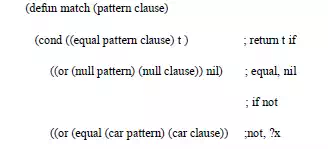
· When a segment variable is encountered (the *y), match is recursively executed on the cdrs of both pattern and clause or on the cdr of clause and pattern as *y

matches one or more than one item respectively

Partial Matching

· For many AI applications complete matching between two or more structures is inappropriate

· For example, input representations of speech waveforms or visual scenes may have been corrupted by noise or other unwanted distortions.

· In such cases, we do not want to reject the input out of hand. Our systems should be more tolerant of such problems

· We want our system to be able to find an acceptable or best match between the input and some reference description

· Compensating for Distortions

· Finding an object in a photograph given only a general description of the object is a common problems in vision applications

· For example, the task may be to locate a human face or human body in photographs without the necessity of storing hundreds of specific face templates

· A better approach in this case would be to store a single reference description of the object

· Matching between photographs regions and corresponding descriptions then could be approached using either a measure of correlation, by altering the image

             to obtain a closer fit

· If nothing is known about the noise and distortion characteristics, correlation methods can be ineffective or even misleading. In such cases, methods based on

mechanical distortion may be appropriate

· For example, our reference image is on a transparent rubber sheet. This sheet is moved over the input image and at each location is stretched to get the best

match alignment between the two images

· The match between the two can then be evaluated by how well they correspond and how much push-and-pull distortion is needed to obtain the best correspondence

· Use the number of rigid pieces connected with springs. This pieces can correspond to low level areas such as pixels or even larger area segments

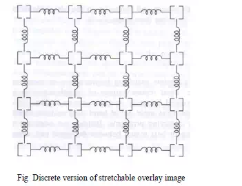
· To model any restrictions such as the relative positions of body parts, nonlinear cost functions of piece displacements can be used

· The costs can correspond to different spring tensions which reflect the constraints

· For example, the cost of displacing some pieces might be zero for no displacement, one unit for single increment displacements in any one of the permissible directions, two units for two position displacements and infinite cost for displacements of more than two increments. Other pieces would be assigned higher costs for unit and larger position displacements when stronger constraints were applicable

· The matching problem is to find a least cost location and distortion pattern for the reference sheet with regard to the sensed picture

· Attempting to compare each component of some reference to each primitive part of a sensed picture is a combinatorially explosive problem

· In using the template-spring reference image and heuristic methods to compare against different segments of the sensed picture, the search and match process

             can be made tractable

· Any matching metric used in the least cost comparison would need to take into account the sum of the distortion costs Cd , the sum of the costs for reference and

            sensed component dissimilarities Cc , and the sum of penalty costs for missing components Cm . Thus, the total cost is given by

          Ct = Cd + Cc + Cm

Finding Match Differences

· Distortions occurring in representations are not the only reason for partial matches

· For example, in problem solving or analogical inference, differences are expected. In such cases the two structures are matched to isolate the differences in order that they may be reduced or transformed. Once again, partial matching techniques are appropriate

· In visual application, an industrial part may be described using a graph structure where the set of nodes correspond to rectangular or cylindrical block subparts

· The arc in the graph correspond to positional relations between the subparts

· Labels for rectangular block nodes contain length, width and height, while labels for cylindrical block nodes, where location can be above, to the right of, behind,

inside and so on

· In Fig 8.5 illustrates a segment of such a graph

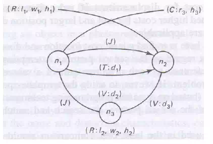
· In the fig the following abbreviations are used

· Interpreting the graph, we see it is a unit consisting of subparts, mode up of rectangular and cylindrical blocks with dimensions specified by attribute values

· The cylindrical block n1 is to the right of n2 by d1 units and the two are connected by a joint

· The blocks n1 and n2 are above the rectangular block n3 by d2 and d3 units respectively, and so on

· Graphs such as this are called attributed relational graphs (ATRs). Such a graph G is defined as a sextuple G = (N, B, A, Gn, Gb)

· Where N = { n1, n2, . . ., nk}is a set of nodes, A = {a n1, an2, . . . , ank} is an alphabet of node attributes, B = { b1, b2, . . . , bm}is a set of directed branches (b = (ni, nj)), and Gn and Gb are functions for generating node and branch attributes respectively

· When the representations are graph structures like ARGs, a similarity measure may be computed as the total cost of transforming one graph into the other

· For example, the similarity of two ARGs may be determined with the following steps:

Ø Decompose the ARGs into basic subgraphs, each having a depth of one

Ø Compute the minimum cost to transform either basic ARG into the other one subgraph-by-subgraph

Ø Compute the total transformation cost from the sum of the subgraph costs

· An ARG may be transformed by the three basic operations of node or branch deletions, insertions, or substitutions, where each operation is given a cost based

on computation time or other factors

The RETE matching algorithm

· One potential problem with expert systems is the number of comparisons that need to be made between rules and facts in the database.

· In some cases, where there are hundreds or even thousands of rules, running comparisons against each rule can be impractical.

· The Rete Algorithm is an efficient method for solving this problem and is used by a number of expert system tools, including OPS5 and Eclipse.

· The Rete is a directed, acyclic, rooted graph.

· Each path from the root node to a leaf in the tree represents the left-hand side of a rule.

· Each node stores details of which facts have been matched by the rules at that point in the path. As facts are changed, the new facts are propagated through the Rete from the root node to the leaves, changing the information stored at nodes appropriately.

· This could mean adding a new fact, or changing information about an old fact, or deleting an old fact. In this way, the system only needs to test each new fact against

the rules, and only against those rules to which the new fact is relevant, instead of checking each fact against each rule.

· The Rete algorithm depends on the principle that in general, when using forward chaining in expert systems, the values of objects change relatively infrequently,

              meaning that relatively few changes need to be made to the Rete.

· In such cases, the Rete algorithm can provide a significant improvement in performance over other methods, although it is less efficient in cases where objects

are continually changing.

· The basic inference cycle of a production system is match, select and execute as indicated in Fig 8.6. These operations are performed as follows

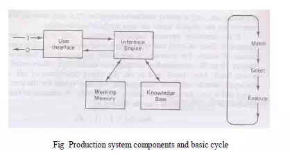
Match

· During the match portion of the cycle, the conditions in the LHS of the rules in the knowledge base are matched against the contents of working memory to determine which rules have their LHS conditions satisfied with consistent bindings to working memory terms.

· Rules which are found to be applicable are put in a conflict set

Select

· From the conflict set, one of the rules is selected to execute. The selection strategy may depend on recency of useage, specificity of the rule or other criteria

Execute

· The rule selected from the conflict set is executed by carrying the action or conclusion part of the rule, the RHS of the rule. This may involve an I/O operation, adding, removing or changing clauses in working memory or simply causing a halt

· The above cycle is repeated until no rules are put in the conflict set or until a stopping condition is reached

· The main time saving features of RETE are as follows

1. in most expert systems, the contents of working memory change verylittle from cycle to cycle. There is persistence in the data known as temporal redundancy. This makes exhaustive matching on every cycle unnecessary. Instead, by saving match information, it is only necessary to compare working memory changes on each cycle. In RETE,

addition to, removal from, and changes to working memory are  translated directly into changes to the conflict set in Fig . Then when a rule from the conflict set has been selected to fire, it is removed from the set and the remaining entries are saved for the next cycle. Consequently, repetitive matching of all rules against working memory

is avoided. Furthermore, by indexing rules with the condition terms appearing in their LHS, only those rules which could match. Working memory changes need to be examined. This greatly reduces the number of comparisons required on each cycle

2. Many rules in a knowledge base will have the same conditions occurring in their LHS. This is just another way in which unnecessary matching can arise. Repeating testing of the same conditions in those rules could be avoided by grouping rules which share the same conditions and linking them to their common terms. It would then be

possible to perform a single set of tests for all the applicable rules shown in Fig below