Uniformed or Blind search

Breadth First Search (BFS):

BFS expands the leaf node with the lowest path cost so far, and keeps going until a goal node is generated. If the path cost simply equals the number of links, we can implement this as a simple queue (“first in, first out”).

Ø This is guaranteed to find an optimal path to a goal state. It is memory intensive if the state space is large. If the typical branching factor is b, and the depth of the shallowest goal state is d – the space complexity is O(bd), and the time complexity is O(bd).

Ø BFS is an easy search technique to understand. The algorithm is presented below.

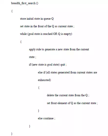
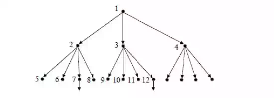
Ø The algorithm is illustrated using the bridge components configuration problem. The initial state is PDFG, which is not a goal state; and hence set it as the current state. Generate another state DPFG (by swapping 1st and 2nd position values) and add it to the list. That is not a goal state, hence; generate next successor state, which is FDPG (by swapping 1st and 3rd position values). This is also not a goal state; hence add it to the list and generate the next successor state GDFP.

Ø Only three states can be generated from the initial state. Now the queue Q will have three elements in it, viz., DPFG, FDPG and GDFP. Now take DPFG (first state in the list) as the current state and continue the process, until all the states generated from this are evaluated. Continue this process, until the goal state DGPF is reached.

Ø The 14th evaluation gives the goal state. It may be noted that, all the states at one level in the tree are evaluated before the states in the next level are taken up; i.e., the evaluations are carried out breadth-wise. Hence, the search strategy is called breadthfirst search.

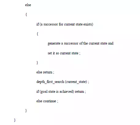
Ø Depth First Search (DFS): DFS expands the leaf node with the highest path cost so far, and keeps going until a goal node is generated. If the path cost simply equals the number of links, we can implement this as a simple stack (“last in, first out”).

· This is not guaranteed to find any path to a goal state. It is memory efficient even if the state space is large. If the typical branching factor is b, and the maximum depth of the tree is m – the space complexity is O(bm), and the time complexity is O(bm).

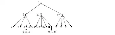
· In DFS, instead of generating all the states below the current level, only the first state below the current level is generated and evaluated recursively. The search continues till a further successor cannot be generated.

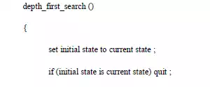
· Then it goes back to the parent and explores the next successor. The algorithm is given below.

· Since DFS stores only the states in the current path, it uses much less memory during the search compared to BFS.

· The probability of arriving at goal state with a fewer number of evaluations is higher with DFS compared to BFS. This is because, in BFS, all the states in a level have to be evaluated before states in the lower level are considered. DFS is very efficient when more acceptable solutions exist, so that the search can be terminated once the first acceptable solution is obtained.

· BFS is advantageous in cases where the tree is very deep.

· An ideal search mechanism is to combine the advantages of BFS and DFS.

· Depth Limited Search (DLS): DLS is a variation of DFS. If we put a limit l on how deep a depth first search can go, we can guarantee that the search will terminate (either in success or failure).

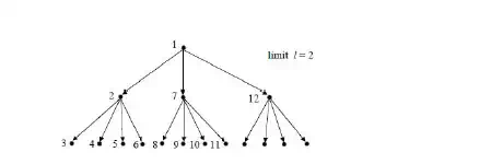
· If there is at least one goal state at a depth less than l, this algorithm is guaranteed to find a goal state, but it is not guaranteed to find an optimal path. The space complexity is O(bl), and the time complexity is O(bl).

· Depth First Iterative Deepening Search (DFIDS): DFIDS is a variation of DLS. If the lowest depth of a goal state is not known, we can always find the best limit l for

DLS by trying all possible depths l = 0, 1, 2, 3, … in turn, and stopping once we have achieved a goal state.

· This appears wasteful because all the DLS for l less than the goal level are useless, and many states are expanded many times. However, in practice, most of the time is spent at the deepest part of the search tree, so the algorithm actually combines the benefits of DFS and BFS.

· Because all the nodes are expanded at each level, the algorithm is complete and optimal like BFS, but has the modest memory requirements of DFS. Exercise: if we

had plenty of memory, could/should we avoid expanding the top level states many times?

· The space complexity is O(bd) as in DLS with l = d, which is better than BFS.

· The time complexity is O(bd) as in BFS, which is better than DFS.

· Bi-Directional Search (BDS): The idea behind bi-directional search is to search simultaneously both forward from the initial state and backwards from the goal state,

and stop when the two BFS searches meet in the middle.

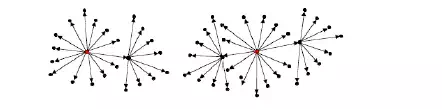
· This is not always going to be possible, but is likely to be feasible if the state transitions are reversible. The algorithm is complete and optimal, and since the two

search depths are ~d/2, it has space complexity O(bd/2), and time complexity O(bd/2). However, if there is more than one possible goal state, this must be factored into the complexity.

· Repeated States: In the above discussion we have ignored an important complication that often arises in search processes – the possibility that we will waste time by expanding states that have already been expanded before somewhere else on the search tree.

· For some problems this possibility can never arise, because each state can only be reached in one way.

· For many problems, however, repeated states are unavoidable. This will include all problems where the transitions are reversible, e.g.

· The search trees for these problems are infinite, but if we can prune out the repeated states, we can cut the search tree down to a finite size, We effectively only generate a

portion of the search tree that matches the state space graph.

· Avoiding Repeated States: There are three principal approaches for dealing with repeated states:

· Never return to the state you have just come from The node expansion function must be prevented from generating any node successor that is the same state as the node’s parent.

· Never create search paths with cycles in them The node expansion function must be prevented from generating any node successor that is the same state as any of the node’s ancestors.

· Never generate states that have already been generated before This requires that every state ever generated is remembered, potentially resulting in space complexity of O(bd).

· Comparing the Uninformed Search Algorithms: We can now summarize the properties of our five uninformed search strategies:

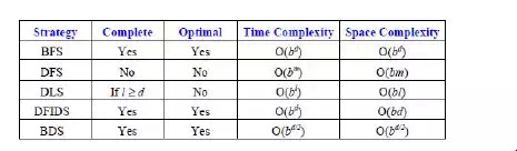
· Simple BFS and BDS are complete and optimal but expensive with respect to space and time.

· DFS requires much less memory if the maximum tree depth is limited, but has no guarantee of finding any solution, let alone an optimal one. DLS offers an improvement over DFS if we have some idea how deep the goal is.

· The best overall is DFID which is complete, optimal and has low memory requirements, but still exponential time.

Informed search

Ø Informed search uses some kind of evaluation function to tell us how far each expanded state is from a goal state, and/or some kind of heuristic function to help us decide which state is likely to be the best one to expand next.

Ø The hard part is to come up with good evaluation and/or heuristic functions. Often there is a natural evaluation function, such as distance in miles or number objects in the wrong position.

Ø Sometimes we can learn heuristic functions by analyzing what has worked well in similar previous searches.

Ø The simplest idea, known as greedy best first search, is to expand the node that is already closest to the goal, as that is most likely to lead quickly to a solution. This is like DFS in that it attempts to follow a single route to the goal, only attempting to try a different route when it reaches a dead end. As with DFS, it is not complete, not optimal, and has time and complexity of O(bm). However, with good heuristics, the time complexity can be reduced substantially.

Ø Branch and Bound: An enhancement of backtracking.

Ø Applicable to optimization problems.

Ø For each node (partial solution) of a state-space tree, computes a bound on the value of the objective function for all descendants of the node (extensions of the partial solution).

Ø Uses the bound for:

Ø Ruling out certain nodes as “nonpromising” to prune the tree – if a node’s bound is not better than the best solution seen so far.

Ø Guiding the search through state-space.

Ø The search path at the current node in a state-space tree can be terminated for any one of the following three reasons:

Ø The value of the node’s bound is not better than the value of the best solution seen so far.

Ø The node represents no feasible solutions because the constraints of the problem are already violated.

Ø The subset of feasible solutions represented by the node consists of a single point and hence we compare the value of the objective function for this

feasible solution with that of the best solution seen so far and update the latter with the former if the new solution is better.

Best-First branch-and-bound:

Ø A variation of backtracking.

Ø Among all the nonterminated leaves, called as the live nodes, in the current tree, generate all the children of the most promising node, instead of generation a single child of the last promising node as it is done in backtracking.

Ø Consider the node with the best bound as the most promising node.

A* Search:

Suppose that, for each node n in a search tree, an evaluation function f(n) is defined as the sum of the cost g(n) to reach that node from the start state, plus an

estimated cost h(n) to get from that state to the goal state. That f(n) is then the estimated cost of the cheapest solution through n.

Ø A* search, which is the most popular form of best-first search, repeatedly picks the node with the lowest f(n) to expand next. It turns out that if the heuristic function h(n) satisfies certain conditions, then this strategy is both complete and optimal.

Ø In particular, if h(n) is an admissible heuristic, i.e. is always optimistic and never overestimates the cost to reach the goal, then A* is optimal.

Ø The classic example is finding the route by road between two cities given the straight line distances from each road intersection to the goal city. In this case, the nodes are the intersections, and we can simply use the straight line distances as h(n).

Hill Climbing / Gradient Descent:

The basic idea of hill climbing is simple: at each current state we select a transition, evaluate the resulting state, and if the resulting state is an improvement we move there, otherwise we try a new transition from where we are.

Ø We repeat this until we reach a goal state, or have no more transitions to try. The transitions explored can be selected at random, or according to some problem specific heuristics.

Ø In some cases, it is possible to define evaluation functions such that we can compute the gradients with respect to the possible transitions, and thus compute which

transition direction to take to produce the best improvement in the evaluation function.

Ø Following the evaluation gradients in this way is known as gradient descent.

Ø In neural networks, for example, we can define the total error of the output activations as a function of the connection weights, and compute the gradients of how the error changes as we change the weights. By changing the weights in small steps against those gradients, we systematically minimize the network’s output errors.