Search and Control Strategies:

Problem solving is an important aspect of Artificial Intelligence. A problem can be considered to consist of a goal and a set of actions that can be taken to lead to the goal. At any given time, we consider the state of the search space to represent where we have reached as a result of the actions we have applied so far. For example, consider the problem of looking for a contact lens on a football field. The initial state is how we start out, which is to say we know that the lens is somewhere on the field, but we don’t know where. If we use the representation where we examine the field in units of one square foot, then our first action might be to examine the square in the top-left corner of the field. If we do not find the lens there, we could consider the state now to be that we have examined the top-left square and have not found the lens. After a number of actions, the state might be that we have examined 500 squares, and we have now just found the lens in the last square we examined. This is a goal state because it satisfies the goal that we had of finding a contact lens.

Search is a method that can be used by computers to examine a problem space like this in order to find a goal. Often, we want to find the goal as quickly as possible or without using too many resources. A problem space can also be considered to be a search space because in order to solve the problem, we will search the space for a goal state.We will continue to use the term search space to describe this concept. In this chapter, we will look at a number of methods for examining a search space. These methods are called search methods.

· The Importance of Search in AI

Ø It has already become clear that many of the tasks underlying AI can be phrased in terms of a search for the solution to the problem at hand.

Ø Many goal based agents are essentially problem solving agents which must decide what to do by searching for a sequence of actions that lead to their solutions.

Ø For production systems, we have seen the need to search for a sequence of rule applications that lead to the required fact or action.

Ø For neural network systems, we need to search for the set of connection weights that will result in the required input to output mapping.

· Which search algorithm one should use will generally depend on the problem domain? There are four important factors to consider:

Ø Completeness – Is a solution guaranteed to be found if at least one solution exists?

Ø Optimality – Is the solution found guaranteed to be the best (or lowest cost) solution if there exists more than one solution?

Ø Time Complexity – The upper bound on the time required to find a solution, as a function of the complexity of the problem.

Ø Space Complexity – The upper bound on the storage space (memory) required at any point during the search, as a function of the complexity of the problem.

Preliminary concepts

· Two varieties of space-for-time algorithms:

Ø Input enhancement — preprocess the input (or its part) to store some info to be used later in solving the problem o Counting for sorting o String searching algorithms

Ø Prestructuring — preprocess the input to make accessing its elements easier Hashing

Indexing schemes (e.g., B-trees)

· State Space Representations: The state space is simply the space of all possible states, or configurations, that our system may be in. Generally, of course, we prefer to work with some convenient representation of that search space.

· There are two components to the representation of state spaces:

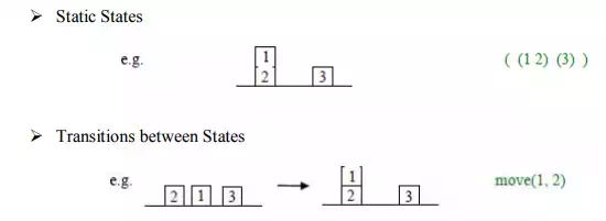
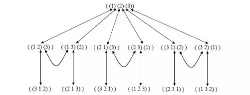
· State Space Graphs: If the number of possible states of the system is small enough, we can represent all of them, along with the transitions between them, in a state space graph, e.g.

· Routes through State Space: Our general aim is to search for a route, or sequence of transitions, through the state space graph from our initial state to a goal state.

· Sometimes there will be more than one possible goal state. We define a goal test to determine if a goal state has been achieved.

· The solution can be represented as a sequence of link labels (or transitions) on the state space graph. Note that the labels depend on the direction moved along the link.

· Sometimes there may be more than one path to a goal state, and we may want to find the optimal (best possible) path. We can define link costs and path costs for measuring the cost of going along a particular path, e.g. the path cost may just equal the number of links, or could be the sum of individual link costs.

· For most realistic problems, the state space graph will be too large for us to hold all of it explicitly in memory at any one time.

· Search Trees: It is helpful to think of the search process as building up a search tree of routes through the state space graph. The root of the search tree is the search node corresponding to the initial state.

· The leaf nodes correspond either to states that have not yet been expanded, or to states that generated no further nodes when expanded.

· At each step, the search algorithm chooses a new unexpanded leaf node to expand. The different search strategies essentially correspond to the different algorithms one can use to select which is the next mode to be expanded at each stage.

Examples of search problems

· Traveling Salesman Problem: Given n cities with known distances between each pair, find the shortest tour that passes through all the cities exactly once before returning to the starting city.

· A lower bound on the length l of any tour can be computed as follows ü For each city i, 1 ≤ i ≤ n, find the sum si of the distances from city i to the two nearest cities. ü Compute the sum s of these n numbers. ü Divide the result by 2 and round up the result to the nearest integer lb = s / 2

· The lower bound for the graph shown in the Fig 5.1 can be computed as follows:

· For any subset of tours that must include particular edges of a given graph, the lower bound can be modified accordingly. E.g.: For all the Hamiltonian circuits of the graph that must include edge (a, d), the lower bound can be computed as follows: lb = [(1 + 5) + (3 + 6) + (1 + 2) + (3 + 5) + (2 + 3)] / 2 = 16.

· Applying the branch-and-bound algorithm, with the bounding function lb = s / 2, to find the shortest Hamiltonian circuit for the given graph, we obtain the state-space tree as shown below:

· To reduce the amount of potential work, we take advantage of the following two observations:

Ø We can consider only tours that start with a.

Ø Since the graph is undirected, we can generate only tours in which b is visited before c.

· In addition, after visiting n – 1 cities, a tour has no choice but to visit the remaining unvisited city and return to the starting one is shown in the Fig 5.2

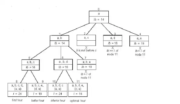
Root node includes only the starting vertex a with a lower bound of

lb = [(1 + 3) + (3 + 6) + (1 + 2) + (3 + 4) + (2 + 3)] / 2 = 14.

Ø Node 1 represents the inclusion of edge (a, b) lb = [(1 + 3) + (3 + 6) + (1 + 2) + (3 + 4) + (2 + 3)] / 2 = 14.

Ø Node 2 represents the inclusion of edge (a, c). Since b is not visited before c, this node is terminated.

Ø Node 3 represents the inclusion of edge (a, d) lb = [(1 + 5) + (3 + 6) + (1 + 2) + (3 + 5) + (2 + 3)] / 2 = 16.

Ø Node 1 represents the inclusion of edge (a, e) lb = [(1 + 8) + (3 + 6) + (1 + 2) + (3 + 4) + (2 + 8)] / 2 = 19.

Ø Among all the four live nodes of the root, node 1 has a better lower bound. Hence we branch from node 1.

Ø Node 5 represents the inclusion of edge (b, c) lb = [(1 + 3) + (3 + 6) + (1 + 6) + (3 + 4) + (2 + 3)] / 2 = 16.

Ø Node 6 represents the inclusion of edge (b, d) lb = [(1 + 3) + (3 + 7) + (1 + 2) + (3 + 7) + (2 + 3)] / 2 = 16.

Ø Node 7 represents the inclusion of edge (b, e) lb = [(1 + 3) + (3 + 9) + (1 + 2) + (3 + 4) + (2 + 9)] / 2 = 19.

Ø Since nodes 5 and 6 both have the same lower bound, we branch out from each of them.

Ø Node 8 represents the inclusion of the edges (c, d), (d, e) and (e, a). Hence, the length of the tour, l = 3 + 6 + 4 + 3 + 8 = 24.

Ø Node 9 represents the inclusion of the edges (c, e), (e, d) and (d, a). Hence, the length of the tour, l = 3 + 6 + 2 + 3 + 5 = 19.

Ø Node 10 represents the inclusion of the edges (d, c), (c, e) and (e, a). Hence, the length of the tour, l = 3 + 7 + 4 + 2 + 8 = 24.

Ø Node 11 represents the inclusion of the edges (d, e), (e, c) and (c, a). Hence, the length of the tour, l = 3 + 7 + 3 + 2 + 1 = 16.

Ø Node 11 represents an optimal tour since its tour length is better than or equal to the other live nodes, 8, 9, 10, 3 and 4.

Ø The optimal tour is a → b → d → e → c → a with a tour length of 16.