Comparison Study of AI-based Methods in Wind Energy
The important environmental advantages of renewable energy sources have been significantly noticed, which results in most industrialized countries committed to developing the installation of wind power plants [1]. The share of total installed capacity of wind power in China has reached approximately 27% in the global capacity, which is 96.37 GW, due to the historically high installation of new wind power capacity.1 Moreover, a renewable-energy-oriented power system was proposed as the fundamental aim of China’s energy transformation during the Asia-Pacific Economic Cooperation (APEC) Conferences.2Advanced prediction techniques are urgently needed to integrate wind energy into the electrical power grid in a manner that benefits both Transmission System Operators (TSOs) and Independent Power Producers (IPPs) [2,3].
Since wind energy has the inherently intermittent nature and stochastic nonstationarity, it brings significant levels of uncertainty to system operators [4]. Thus, accurate wind forecasts are of primary importance to solve operational, planning, and economic problems in the growing wind power scenario [4,5]. Current wind power forecasting research has been divided into point forecasts (also called deterministic predictions) [6–8] and uncertainty forecasts [9,10]. Deterministic forecasts deliver specific amounts of wind power and focus on reducing the forecasting error [11]. By contrast, it is essential to decision-making processes and electricity market trading strategies [12] that uncertainty forecasts provide uncertainty information for system operators to manage the wind power generation of wind farms [11,13].The existing approaches published in the literature with respect to wind energy prediction can be divided into three categories—artificial intelligent model, physical model, and statistical model—and sometimes a hybrid one, which integrates advantages of different categories, is involved. Researchers often utilize them to forecast various types of wind speed and wind power by various types including the multi-step forecasting, long-term wind speed (power) forecasting, and so on. However, few literature exist to discuss an overall comparison among various forecasting types, which is a foundation for future works of wind energy prediction because this comparison may reveal whether there is a best model for a specific forecasting type or specific data in the field of wind energy.The following parts in this paper are demonstrated by four sections: methodology briefly introduces forecasting approaches that this paper adopts; data collection specifically illustrates three types of wind data; simulation and result displays and evaluates the final results of forecasting effectiveness of each model; and conclusion draws the main results that this paper investigates.
Methodology
In this section, we will introduce five basic models including Autoregressive Moving Average Model (ARMA), Back-Propagation Neuron Network (BPNN), Support Vector Regression (SVR), Extreme Learning Machine (ELM), and Adaptive Network-Based Fuzzy Inference System (ANFIS) as forecasting methods in this paper to predict wind speed. For the purpose of clearly demonstrating procedures of forecasting wind speed using these methods, this chapter will attach the Matlab code after introduction of each model and the wind speed series is defined as follows:
where N is a positive integer and wsn∈(0,+∞)⊂Rwsn∈(0,+∞)⊂ℝ represents the wind speed of time n.
AUTOREGRESSIVE MOVING AVERAGE MODEL
BRIEF INTRODUCTION OF ARMA
This section displays ARMA model and the ARMA(p, q) model can be expressed as follows [14]:
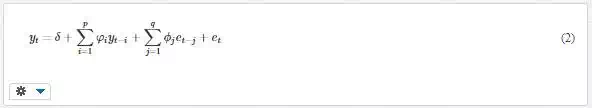
Where δδ is the constant term of the ARMA model, φiφi is the ith autoregressive coefficient, ϕjϕj is the jth moving average coefficient, et is the error term at time period t, and represents the value of wind speed observed or forecasted at time period t. Thus, the first step in applying ARMA model to forecast wind speed is to identify p and q, which is related to the stationarity of the time series, which means that the stationarity assumption of observed series should be checked first. For this purpose, inspection of the run plots and Auto Correlation Function (ACF) plots can be used for deciding on the order of differencing.
IMPLEMENT FOR WIND SPEED FORECASTING
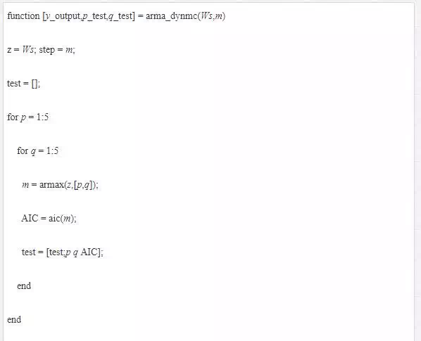
Since the Matlab has the ARMA package, we will implement this model to forecast wind speed using five steps as follows:
1. Identify the domain of p and q. In this chapter, we set p∈{1,2,3,4,5}p∈{1,2,3,4,5} and q∈{1,2,3,4,5}q∈{1,2,3,4,5}.
2. For each pair (p, q), calculate corresponding model’s AIC value.
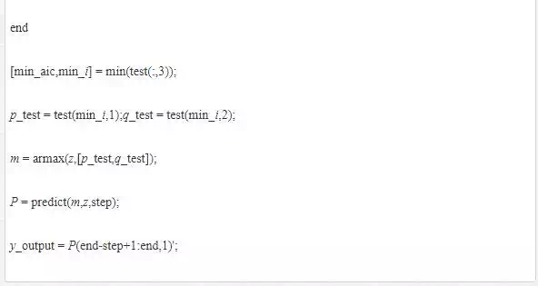
3. Select the pair (p, q), which makes corresponding model’s AIC value to be minimum one among all of pairs of (p, q) as the best (p, q) and denote this pair as (p_test, q_test).
4. Apply (p_test, q_test) to establish ARMA model.
5. Forecast m steps using the model established in step (4).
The detailed Matlab codes are listed in Code 1.
Code 1. Matlab Codes of ARMA.
BACK-PROPAGATION NEURON NETWORK
BRIEF INTRODUCTION OF BPNN
Mccelland and Rumelhart developed the BP neural network model in 1985. There are three layers in a particular network: the input, hidden, and output layers. Each layer has designed nodes, whose functions aim to calculate the inner product of the input vector and weight vector by the transfer function [15]. The process of BPNN is demonstrated by the following steps:
1. Initialize. Assume that the input layer has n nodes, and hidden layer has l nodes, and output layer has m nodes. Let the network distribute values randomly for each threshold value θj, γt and the connection weight wij, vjt, i = 1, 2, …, n, j = 1, 2, …, l, and t = 1, 2, …, m.
2. Calculate the output of hidden layer. Assume X⊂[−1,1]n⊂[−1,1]n is the input space and Y⊂[−1,1]m⊂[−1,1]m is the output space, which means X is an n-dimensional space and Y is an m-dimensional space. We denote each element in as xi and each element in Y is yt. Thus, the output of hidden layer can be calculated using the following function:

f(∙)f(•) is the transfer function and is expressed as follows

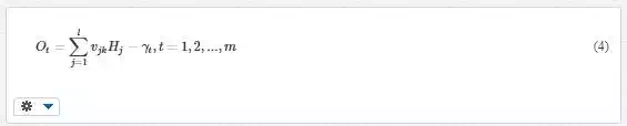
Calculate the output of the network. Using Hj, vjk, and γt, the output of the network can be calculated as follows:
1. Error calculation. The error between yt and Ot can be expressed as et = Ot – yt.
2. Weights updating. According to back-propagation algorithm, the weights wij, vjt can be updated by using the following functions:
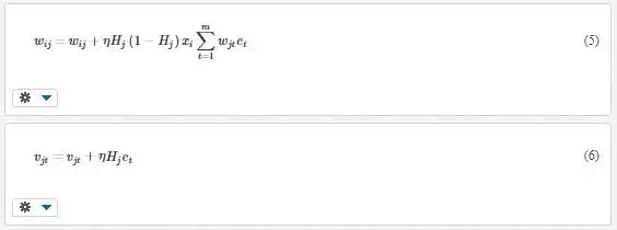
1. where ηη is the learning rate and i = 1, 2, …, n, j = 1, 2, …, l, and t = 1, 2, …, m.
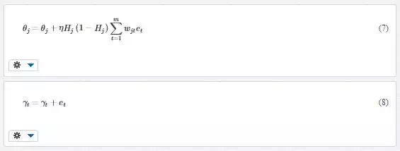
2. Biases updating. Similarly, the biases θj, γt can be updated by using the following functions:
1. Iteration. If the error is more than the expected value, then execute steps (2)–(6). Otherwise, denote θj, γt, wij, and vjt as the optimized parameter of this network with respect to X and Y.
IMPLEMENT FOR WIND SPEED FORECASTING
In this part, how to apply BPNN to forecast wind speed will be introduced in detail and the MATLAB code for predicting wind speed will be attached. There are six steps to forecast wind speed applying BPNN as follows:
1. Design forecasting mode. In this chapter, AI-based model will apply the following mode to forecast wind speed of different wind databases
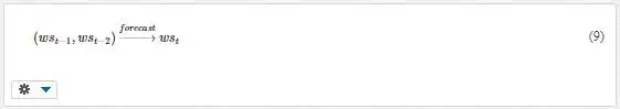
1. Eq. (8) indicates that the input space X for BPNN model is a two-dimensional space and the output space Y is a one-dimensional space, meaning that n = 2 and m = 1 as described in Section 2.2.1.
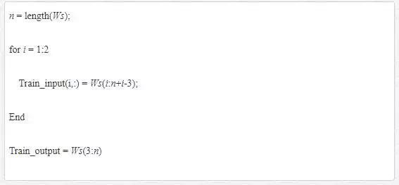
2. Assign training samples. Based on step (1), the input and output of training samples are expressed as follows:
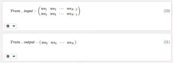
The Matlab codes of this step are listed in Code 2. Code 2. Matlab codes to construct training samples.
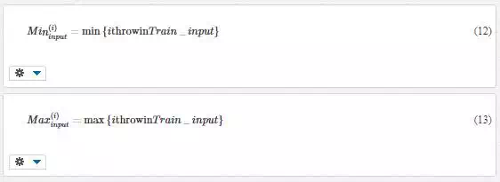
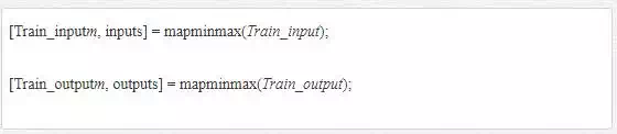
Normalize Train_input and Train_output. Since X⊂[−1,1]nX⊂[−1,1]n and Y⊂[−1,1]mY⊂[−1,1]m, Train_inputand Train_output need to be adjusted to satisfy this condition. First, the maximum and minimum values of each row in Train_input need to be calculated using the following functions:
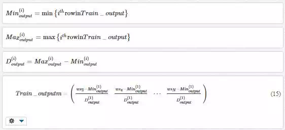
Let D(i)input=Max(i)input−Min(i)inputDinput(i)=Maxinput(i)−Mininput(i) and normalized Train_input can be obtained by the following equation (i = 1, 2):

Similarly, normalized Train_output can be obtained by the following equations:
The Matlab codes of this step are listed in Code 3.
Code 3. Matlab codes to normalize training samples.
Assign parameters and train the network. We assign that the network has three layers and the input layer has two nodes, the hidden layer has two nodes and the output layer has one node. Thus, according to Section 2.2.1, the optimized weights and biases of this network can be calculated and denoted by θj, γt, wij, vjt, i = 1, 2, j = 1, 2, and t = 1. The Matlab codes of this step are listed in Code 4.
Code 4. Matlab codes to build and train BPNN.

1. Net is the trained network and can be applied to forecast wind speed in the following steps:
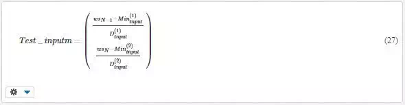
2. Forecast wsN+1wsN+1. Based on the forecasting mode in step (1), we need to apply wsN−1wsN−1 and wsNwsN to forecast wsN+1wsN+1, which means that the Test_input is (wsN−1,wsN)T(wsN−1,wsN)T. Then, D(i)input,Max(i)inputandMin(i)inputDinput(i),Maxinput(i)andMininput(i) obtained in step (3) will be applied to normalize Test_input and the normalized Test_input can be expressed using Test_inputm as follows:
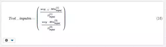
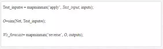
Applying Eqs. (3) and (4) in Section 2.2.1, we can obtain the output of the network and denote it by O∈RO∈ℝ. Thus, the forecasting value of wsN+1wsN+1 is Ws_forecast = O×D(1)output+Min(1)outputO×Doutput(1)+Minoutput(1).The Matlab codes of this step are listed in Code 5.
Code 5. Matlab codes to forecast using established BPNN (single step ahead)
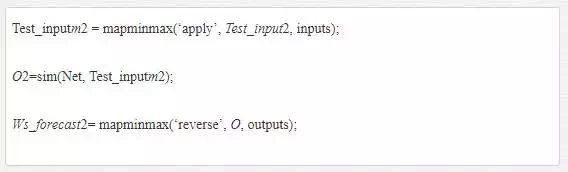
Forecast wsN+2wsN+2. Based on the forecasting mode in step (1), we need to apply wsNwsN and forecasting value of wsN+1wsN+1, Ws_forecast, to forecast wsN+2wsN+2, which means that the Test_input2 is (wsN,Ws_forecast)T(wsN,Ws_forecast)T. Then, D(i)input,Max(i)inputandMin(i)inputDinput(i),Maxinput(i)andMininput(i) obtained in step (3) will be applied to normalize Test_input2 and the normalized Test_input2 can be expressed using Test_inputm2 as follows:

Applying Eqs. (3) and (4) in Section 2.2.1, we can obtain the output of the network and denote it by O2∈RO2∈ℝ. Therefore, the forecasting value of wsN+2wsN+2 is Ws_forecast2 = O2×D(1)output+Min(1)outputO2×Doutput(1)+Minoutput(1).
The Matlab codes of this step are listed in Code 6.
Code 6. Matlab codes to forecast using established BPNN (two-step ahead).
SUPPORT VECTOR REGRESSION
BRIEF INTRODUCTION OF SVR
SVR is the most common application of support vector machines (SVMs) and constructs a hyperplane that separates examples with maximum margin, to categorize or forecast series [16]. Given the training data {(x1,y1),…,(xl,yl)}⊂X×R{(x1,y1),…,(xl,yl)}⊂Χ×ℝ, where X=RdΧ=ℝd denotes the space of input patterns, then the goal of SVR is to find a function f(x)f(x) that is as flat as possible with at most εε deviation from the actually obtained targets yiyi for all the training data. The simplest, linear formula for the output of a linear SVR is defined as [17]
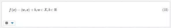
where ⟨w,x⟩〈w,x〉 denotes the dot product in XΧ. One way to get the largest flatness is to minimize the ww in Eq. (18) and this problem can be written as Eq. (19) by introducing slack variables ξiξi, ξ∗iξi* into a convex optimization problem function:
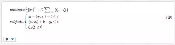
he constant C>0C>0 determines the trade-off between the flatness of f and the amount up to which deviations larger than εε are tolerated.
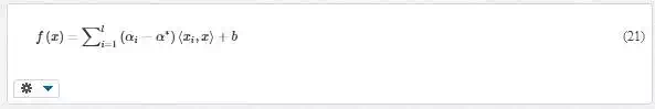
To figure out the support vector regression function, the dual problem of Eq. (19) is defined in Eq. (20)by constructing a Lagrange function from the objective function:

With the solution of (α,α∗)(α,α*) from Eq. (20), the support vector regression function can be written as follows:
When it comes to the nonlinear regression problem, the training patterns xixi can be mapped into a high-dimensional space, where the nonlinear regression problem is transformed into a linear one. The expansion of Eq. (21) is defined as Eq. (22):
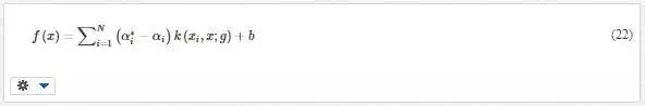
where α∗iαi* and αiαi are Lagrange multipliers and k(xi,x;g)k(xi,x;g) is the kernel function, in which g is a parameter and generally set as 1/d.
IMPLEMENT FOR WIND SPEED FORECASTING
We use the libsvm package (Version 3.17) to implement forecasting task of wind speed using SVR. There are six steps and steps (1)–(3) are same as in steps (1)–(3) in Section 2.2.2. Thus, we start to introduce from step (4).
(4) Assign parameters and train the SVR model. We assign that C is 4 and g is 0.5. Thus, according to Section 2.3.1, the optimized solution (α,α∗)(α,α*) can be calculated. The Matlab codes of this step are listed in Code 7.
Code 7. Matlab codes to establish and train SVR.
Model = svmtrain(Train_output’, Train_input’, ‘-C 4 –g 0.5’);
Model is the trained SVR model and can be applied to forecast wind speed by the following steps:
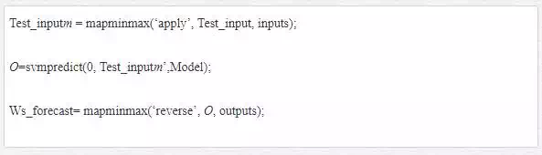
(5) Forecast wsN+1wsN+1. Based on the forecasting mode in step (1), we need to apply wsN−1wsN−1 and wsNwsN to forecast wsN+1wsN+1, which means that the Test_input is (wsN−1,wsN)T(wsN−1,wsN)T. Then, D(i)input,Max(i)inputandMin(i)inputDinput(i),Maxinput(i)andMininput(i) obtained in step (3) will be applied to normalize Test_input and the normalized Test_input can be expressed using Test_inputm as follows:

Applying Eqs. (3) and (4) in Section 2.2.1, we can obtain the output of the network and denote it by O∈RO∈ℝ. Thus, the forecasting value of wsN+1wsN+1 is Ws_forecast = O×D(1)output+Min(1)outputO×Doutput(1)+Minoutput(1). The Matlab codes of this step are listed in Code 8.
Code 8. Matlab codes to forecast using established SVR (single step ahead).
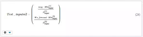
(6) Forecast wsN+2wsN+2. Based on the forecasting mode in step (1), we need to apply wsNwsN and theforecasting value of wsN+1wsN+1, Ws_forecast, to forecast wsN+2wsN+2, which means that the Test_input2 is (wsN,Ws_forecast)T(wsN,Ws_forecast)T. Then, D(i)input,Max(i)inputandMin(i)inputDinput(i),Maxinput(i)andMininput(i) obtained in step (3) will be applied to normalize Test_input2 and the normalized Test_input2 can be expressed using Test_inputm2 as follows:
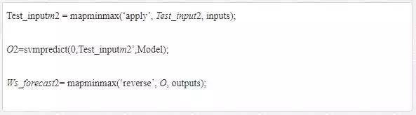
Applying Eqs. (3) and (4) in Section 2.2.1, we can obtain the output of the network and denote it by O2∈RO2∈ℝ. Therefore, the forecasting value of wsN+2wsN+2 is Ws_forecast2 = O2×D(1)output+Min(1)outputO2×Doutput(1)+Minoutput(1). The Matlab codes of this step are listed in Code 9.
Code 9. Matlab codes to forecast using established SVR (two-step ahead).
EXTREME LEARNING MACHINE
BRIEF INTRODUCTION OF ELM
Huang et al. [18] investigated the ELM, which is an effective and efficient learning algorithm. The ELM aims to randomly initialize the weights and biases of SLFN and then to explicitly calculate the hidden layer output matrix and hence the output weights. Because of the nature of non-adjusted weights and bias, the network can be established using a very low computational cost [19]. Then, the ELM with l hidden neurons and transfer function φ(⋅)φ(·) can approximate the N samples with zero error as
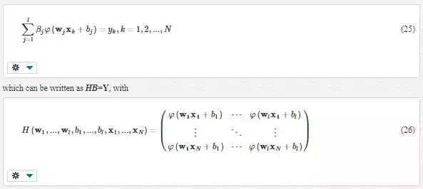
where wi is the weight vector connecting the ith hidden neuron and the input nodes, βiβi is the weight vector connecting the ith hidden neuron and the output neurons, and bibi is the threshold of the ith hidden neuron, and B=(βT1…βTl)T,Y=(yT1…yTN)TB=(β1T…βlT)T,Y=(y1T…yNT)T
Then, the output weights B can be calculated from the hidden layer output matrix H and the target values Y as B^ = H†Y, where H† is the Moore-Penrose generalized inverse of the matrix H.
IMPLEMENT FOR WIND SPEED FORECASTING
We use Matlab to compile ELM model and provide two *.m files, which are Elmtrain.m and Elmpredict.m, in Appendix. Elmtrain function is similar to train function for BPNN and svmtrain function for SVR and Elmpredict function is similar to sim function for BONN and svmpredict function for SVR. In detail, there are six steps for forecasting wind speed using ELM model and steps (1)–(3) are same as in steps (1)(3) in Section 2.2.2. Thus, we start to introduce them from step (4).
(4) Assign parameters and train the ELM model. We design that the input layer of ELM model has two nodes, and the hidden layer of ELM has two nodes, and the output layer of ELM model has one node. Thus, according to Section 2.4.1, the optimized B can be calculated. The Matlab codes of this step are listed in Code 10.
Code 10. Matlab codes to establish and train ELM.
[W,b,B,TF,TYPE] = elmtrain(Train_input, Train_output, 2);
W is the weight matrix of the input layer and hidden layer, and b is the bias vector of input layer and hidden layer, and B is B^ in Section 2.4.1, and TF is the transfer function φ(⋅)φ(·), and TYPE is model’s functions (classification or regression). We select sigmoid function as the transfer function φ(⋅)φ(·) of ELM, which is same as that of BPNN.
(5) Forecast wsN+1wsN+1. Based on the forecasting mode in step (1), we need to apply wsN−1wsN−1 and wsNwsN to forecast wsN+1wsN+1, which means that the Test_input is (wsN−1,wsN)T(wsN−1,wsN)T. Then, D(i)input,Max(i)inputandMin(i)inputDinput(i),Maxinput(i)andMininput(i) obtained in step (3) will be applied to normalize Test_input and the normalized Test_input can be expressed using Test_inputm as follows:
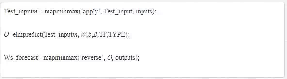
Applying Eqs. (3) and (4) in Section 2.2.1, we can obtain the output of the network and denote it by O∈RO∈ℝ. Thus, the forecasting value of wsN+1wsN+1 is Ws_forecast = O×D(1)output+Min(1)outputO×Doutput(1)+Minoutput(1). The Matlab codes of this step are listed in Code 11.
Code 11. Matlab codes to forecast using established ELM (single step ahead).
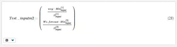
(6) Forecast wsN+2wsN+2. Based on the forecasting mode in step (1), we need to apply wsNwsN and forecasting value of wsN+1wsN+1, Ws_forecast, to forecast wsN+2wsN+2, which means that the Test_input2 is (wsN,Ws_forecast)T(wsN,Ws_forecast)T. Then, D(i)input,Max(i)inputandMin(i)inputDinput(i),Maxinput(i)andMininput(i) obtained in step (3) will be applied to normalize Test_input2 and the normalized Test_input2 can be expressed using Test_inputm2 as follows:
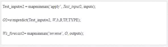
Applying Eqs. (3) and (4) in Section 2.2.1, we can obtain the output of the network and denote it by O2∈RO2∈ℝ. Therefore, the forecasting value of wsN+2wsN+2 is Ws_forecast2 = O2×D(1)output+Min(1)outputO2×Doutput(1)+Minoutput(1). The Matlab codes of this step are listed in Code 12.
Code 12. Matlab codes to forecast using established ELM (two-step ahead).
ADAPTIVE NETWORK-BASED FUZZY INFERENCE SYSTEM
BRIEF INTRODUCTION OF ANFIS
ANFIS is introduced to compensate for the disability of conventional mathematical tools to address uncertain systems, such as human knowledge and reasoning processes. There are two contributions of FIFs restructured: proposing a standard method for transforming ill-defined factors into identifiable rules of FIS and using an adaptive network to tune the membership functions. We assume that there are two fuzzy if-then rules contained in the system, two inputs (x and y) and one output (z), and the processes of ANFIS are described in Figure 1 [20–21].
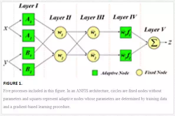
Layer I: Mapping a certain input x to a fuzzy set O(1)iOi(1) for every node i by the member functions μAμA, which is usually bell-shaped with a parameter set {ai,bi,ci}{ai,bi,ci}, as is y

Layer II: In this layer, each circle node performs the connection “AND” and multiplies inputs, as well as sends the product out:

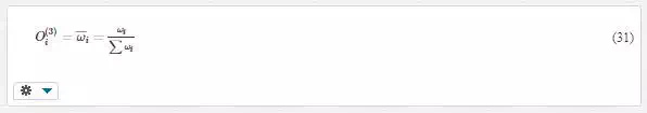
Layer III: Every circle node in this layer calculates a normalized firing strength, namely a ratio of the rule’s firing strength to the sum of all rules’ firing strengths:
Layer IV: Assume the rules of this system are as follows:
Rule 1: If x is A1 and y is B1, then f1=p1x+q1y+r1f1=p1x+q1y+r1
Rule 2: If x is A2 and y is B2, then f2=p2x+q2y+r2f2=p2x+q2y+r2
Then, the outputs of the adaptive nodes in this layer are computed by
|
O(4)i=ω¯¯ifi=ω¯¯i(p1x+q1y+r1)Oi(4)=ω¯ifi=ω¯i(p1x+q1y+r1) |
(32) |
Options
Layer V: The overall output is the weighted average of all incoming signals:
|
(33) |
Options
Particularly, in this case,
|
O(5)i=∑i=12ω¯¯ifi=∑i=12(ω¯¯ix)pi+(ω¯¯iy)qi+ω¯¯iriOi(5)=∑i=12ω¯ifi=∑i=12(ω¯ix)pi+(ω¯iy)qi+ω¯iri |
(34) |
Options
IMPLEMENT FOR WIND SPEED FORECASTING
We use the genfis3 function and ANFIS function in Matlab to implement forecasting task of wind speed using ANFIS. There are six steps and steps (1)–(3) are same as in steps (1)–(3) in Section 2.2.2. Thus, we start to introduce from step (4).
(4) Assign parameters and train the ANFIS model. We set the number of iteration of ANFIS as 100. Thus, the optimized parameters can be calculated. The Matlab codes of this step are listed in Code 13.
Code 13. Matlab codes to establish and train ANFIS.
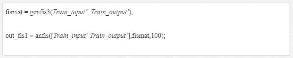
The out_fis1 is the trained ANFIS and can be applied to forecast wind speed.
(5) Forecast wsN+1wsN+1. Based on the forecasting mode in step (1), we need to apply wsN−1wsN−1 and wsNwsN to forecast wsN+1wsN+1, which means that the Test_input is (wsN−1,wsN)T(wsN−1,wsN)T. Then, D(i)input,Max(i)inputandMin(i)inputDinput(i),Maxinput(i)andMininput(i) obtained in step (3) will be applied to normalize Test_input and the normalized Test_input can be expressed using Test_inputm as follows:
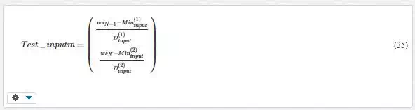
Applying Eqs. (3) and (4) in Section 2.2.1, we can obtain the output of the network and denote it by O∈RO∈ℝ. Thus, the forecasting value of wsN+1wsN+1 is Ws_forecast = O×D(1)output+Min(1)outputO×Doutput(1)+Minoutput(1). The Matlab codes of this step are listed in Code 14.
Code 14. Matlab codes to forecast using established ANFIS (single step ahead).
Test_inputm = mapminmax(‘apply’, Test_input, inputs);
O=evalfis(Test_inputm’, out_fis1);
Ws_forecast= mapminmax(‘reverse’, O, outputs);
(6) Forecast wsN+2wsN+2. Based on the forecasting mode in step (1), we need to apply wsNwsN and forecasting value of wsN+1wsN+1, Ws_forecast, to forecast wsN+2wsN+2, which means that the Test_input2 is (wsN,Ws_forecast)T(wsN,Ws_forecast)T. Then, D(i)input,Max(i)inputandMin(i)inputDinput(i),Maxinput(i)andMininput(i) obtained in step (3) will be applied to normalize Test_input2 and the normalized Test_input2 can be expressed using Test_inputm2 as follows

Applying Eqs. (3) and (4) in Section 2.2.1, we can obtain the output of the network and denote it by O2∈RO2∈ℝ. Therefore, the forecasting value of wsN+2wsN+2 is Ws_forecast2 = O2×D(1)output+Min(1)outputO2×Doutput(1)+Minoutput(1). The Matlab codes of this step are listed in Code 15.
Code 15. Matlab codes to forecast using established ANFIS (two-step ahead).
Test_inputm2 = mapminmax(‘apply’, Test_input2, inputs);
O2=evalfis(Test_inputm2’, out_fis1);
Ws_forecast2= mapminmax(‘reverse’, O, outputs);
Data collection
We select three types of wind data to train and test forecasting models, which are 10-minute wind speed data in wind farm A (this database is denoted by WFD1), 15-minute wind speed data in wind farm B (this database is denoted by WFD2), and 15-minute wind speed data in wind farm C (this database is denoted by WFD3), and wind farms B and C are in the same city in China

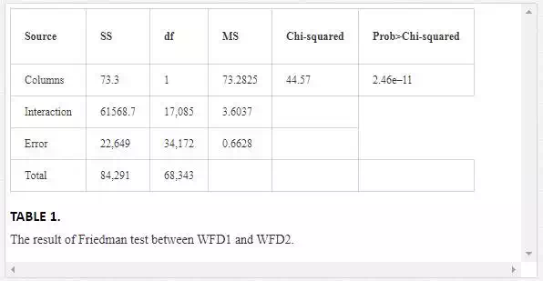
In this section, the descriptive information of each database will be provided and we will test the similarity between WFD2 and WFD3 using Friedman test. In the beginning, Figure 2 shows the three databases and their histograms.
From Figure 2, this is apparent that WFD1 and WFD2 have similar maximum and minimum values because they are in the same city. However, WFD1 and WFD2 have different mean and variance values. Thus, we use Friedman test to figure out whether both of two time series are significantly different, which is shown in Table 1. In Table 1, the p-value of Friedman test is very small (2.46e–11), which indicates that WFD1 and WFD2 have a significant difference.
For WFD3, its mean value is significantly different from others and the histogram of WFD3 is also different from those of other databases. From the description of these three databases, it can be seen that they are very different, which lays a strong foundation for the comparison study.
Simulation and results
For these different databases, we will test 1-h-ahead, 4-h-ahead, 1-h average, 4-h average, and 1-day average wind speed forecasting effectiveness by using five methods separately, which is to say that we conduct five experiments of different time scales or time horizons in this comparison study. To test the overall forecasting effectiveness of each model, the testing period is 30 weeks in 2014 and we apply three criteria to evaluate forecasting error, which are the mean absolute percent error (MAPE), root-mean-squared error (RMSE), and mean absolute error (MAE). The formulas of three criteria are expressed as follows:

where t represents the time t, ytyt is the actual value in time t, yˆty^t is the forecasting value in time t, and N is the length of testing period.
EXPERIMENT I: 1-H-AHEAD WIND SPEED FORECASTING
In this experiment, we will test the 1-h-ahead forecasting effectiveness of five models. It should be pointed that 1-h-ahead prediction means a four-step forecast for WFD1 and WFD2 and a means six-step forecast for WFD3 because WFD3 is constructed by 10-min wind speeds. The main results are shown in Table 2, which contains MAPE, RMSE, and MAE of each model when forecasting 1-h-ahead wind speed.
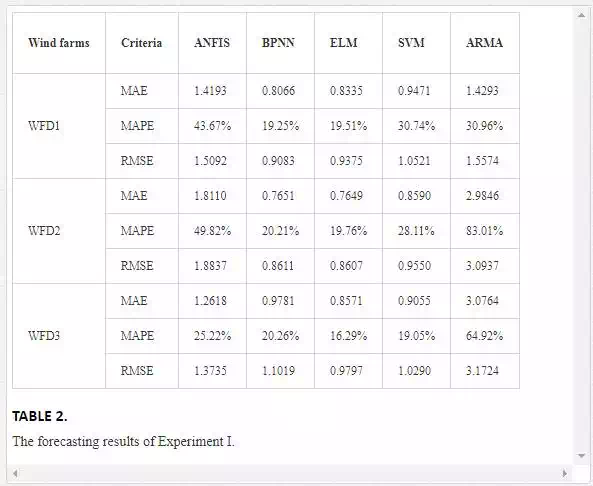
From Table 2, it is apparent that BPNN has the best performance among these five models in WFD1 and ELM outperforms others in WFD2 and WFD3 by three criteria. By contrast, the forecasting accuracy of ANFSI and ARMA is poor and even cannot be accepted in some wind farms, such as the performance of ARMA in WFD1 and WFD2 and the performance of ANFIS in WFD1 and WFD2. These results show that each wind farm has the corresponding best forecasting model and there is no single model that can perform best in every wind farm by three criteria.
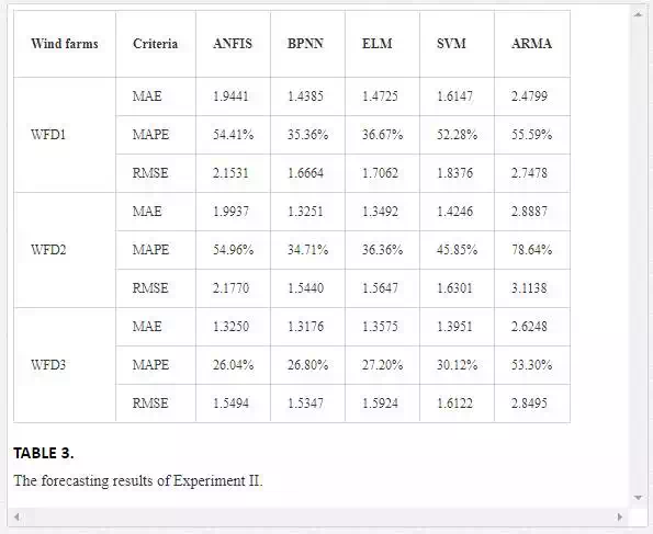
EXPERIMENT II: 4-H-AHEAD WIND SPEED FORECASTING
Experiment II shows the 4-h-ahead forecasting effectiveness of wind speed, and the 4-h-ahead forecasting is equal to a 16-step forecast for WFD1 and WFD2 and is a 24-step forecast for WFD3. Table 3 descripts forecasting results of five models in three wind farms.
In Table 3, BPNN is the best model in WFD1 and WFD2 by three criteria and outperforms other models in three databases by MAE and RMSE. ANFIS has the lowest MAPE in WFD3 among these models but has high MAPE, MAE, and RMSE in WFD1 and WFD2. It is similar to Experiment I that ARMA does not have a decent forecasting results in three wind farms. These results indicate that models forecasting effectiveness varies a lot when the wind farm changes (such as the effectiveness of ANFIS).
EXPERIMENT III: 1-H AVERAGE WIND SPEED FORECASTING
In Experiment III, we will forecast 1-h average wind speed in three wind farms using ANFIS, BPNN, ELM, SVM, and ARMA, and 1-h average wind speed forecasting is a one-step forecast for three wind farms.3 Table 4 shows the forecasting effectiveness of each model in this experiment.

From Table 4, ELM and SVM have decent forecasting accuracy in WFD3, but ELM is better than SVM and other models in WFD1 and WFD2. ANFIS has a good performance in WFD3 and cannot forecast 1-h average wind speed with a reasonable accuracy. Similarly for ARMA, it works well in WFD1 and WFD3 but has a high MAPE in WFD2.
EXPERIMENT IV: 4-H AVERAGE WIND SPEED FORECASTING
It is similar to Experiment III, but this experiment shows the one-step-ahead wind speed forecasting effectiveness of each model. Table 5 demonstrates the results of five models obtained in three wind farms.
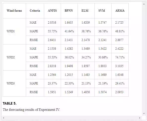
The analyzing results in Table 5 are quite different from that in Table 4. Specifically, SVM model has better performance in WFD1 and WFD2 than other models, and ELM is the best forecasting model in WFD3. For each model, wind speed in WFD3 can be forecasted more accurately than that in WFD1 and WFD2, and AI-based models (ANFIS, BPNN, ELM, and SVM) outperform ARMA in WFD3.
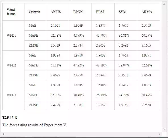
EXPERIMENT V: 1-DAY AVERAGE WIND SPEED FORECASTING
In this experiment, we will test the one-step-ahead forecasting effectiveness based on 1-day average wind speed database. Similar to other experiments, Table 6 demonstrates each model's forecasting effectiveness.
Table 6 shows that SVM has the best forecasting performance on three criteria in three wind farms. By contrast, ARMA and ANFIS have the higher MAPE, MAE, and RMSE than other models.
Conclusion
The inherently intermittent nature and stochastic nonstationarity of wind sources bring great levels of uncertainty to system operators and are an urgent problem in the wind-forecasting field. This chapter introduces some basic forecasting approaches and corresponding procedures to forecast wind speed (detailed codes are attached). After simulating these methods (the testing period is 30 weeks) in MATLAB based on three databases, conclusions can be drawn as follows:
1. None of ANFIS, BPNN, ELM, SVM, and ARMA has the best forecasting performance in all experiments.
2. Based on the experimental results of different forecasting types (1-h-ahead forecasting, 4-h-ahead forecasting, 1-h-average-ahead forecasting, 4-h-average-ahead forecasting, and 1-day-average-ahead forecasting), the best model varies in time scales and time horizons.
3. The forecasting effectiveness differs a lot from database to database (in Experiment II, ANFIS is the best model of which MAPE is 26.04 in WFD3 but has a high MAPE, 54.41%, in WFD1).
4. AI-based models are more suitable for wind speed forecast than ARMA.
According to these conclusions, it is obvious that wind speed forecasting models or systems need to be built up under specific conditions in wind farms and model selection in wind speed forecasting plays a significant role to improve the accuracy.