Turbulence

In fluid dynamics, turbulence or turbulent flow is any pattern of fluid motion characterized by chaotic changes in pressure and flow velocity. It is in contrast to a laminar flow regime, which occurs when a fluid flows in parallel layers, with no disruption between those layers. Turbulence is commonly observed in everyday phenomena such as surf, fast flowing rivers, billowing storm clouds, or smoke from a chimney, and most fluid flows occurring in nature and created in engineering applications are turbulent.  Turbulence is caused by excessive kinetic energy in parts of a fluid flow, which overcomes the damping effect of the fluid's viscosity. For this reason turbulence is easier to create in low viscosity fluids, but more difficult in highly viscous fluids. In general terms, in turbulent flow, unsteady vortices appear of many sizes which interact with each other, consequently drag due to friction effects increases. This would increase the energy needed to pump fluid through a pipe, for instance. However this effect can also be exploited by devices such as aerodynamic spoilers on aircraft, which deliberately "spoil" the laminar flow to increase drag and reduce lift.

The onset of turbulence can be predicted by a dimensionless constant called the Reynolds number, which calculates the balance between kinetic energy and viscous damping in a fluid flow. However, turbulence has long resisted detailed physical analysis, and the interactions within turbulence create a very complex phenomenon. Richard Feynman has described turbulence as the most important unsolved problem in classical physics.

Examples of turbulence

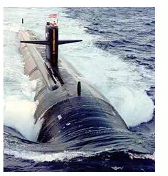
Laminar and turbulent water flow over the hull of a submarine. As the relative velocity of the water increases turbulence occurs

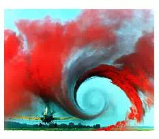
Turbulence in the tip vortex from an airplane wing

· Smoke rising from a cigarette is mostly turbulent flow. However, for the first few centimeters the flow is laminar. The smoke plumebecomes turbulent as its Reynolds number increases, due to its flow velocity and characteristic length increasing.

· Flow over a golf ball. (This can be best understood by considering the golf ball to be stationary, with air flowing over it.) If the golf ball were smooth, the boundary layer flow over the front of the sphere would be laminar at typical conditions. However, the boundary layer would separate early, as the pressure gradient switched from favorable (pressure decreasing in the flow direction) to unfavorable (pressure increasing in the flow direction), creating a large region of low pressure behind the ball that creates high form drag. To prevent this from happening, the surface is dimpled to perturb the boundary layer and promote transition to turbulence. This results in higher skin friction, but moves the point of boundary layer separation further along, resulting in lower form drag and lower overall drag.

· Clear-air turbulence experienced during airplane flight, as well as poor astronomical seeing (the blurring of images seen through the atmosphere.)

· Most of the terrestrial atmospheric circulation

· The oceanic and atmospheric mixed layers and intense oceanic currents.

· The flow conditions in many industrial equipment (such as pipes, ducts, precipitators, gas scrubbers, dynamic scraped surface heat exchangers, etc.) and machines (for instance, internal combustion engines and gas turbines).

· The external flow over all kind of vehicles such as cars, airplanes, ships and submarines.

· The motions of matter in stellar atmospheres.

· A jet exhausting from a nozzle into a quiescent fluid. As the flow emerges into this external fluid, shear layers originating at the lips of the nozzle are created. These layers separate the fast moving jet from the external fluid, and at a certain critical Reynolds number they become unstable and break down to turbulence.

· Biologically generated turbulence resulting from swimming animals affects ocean mixing.

· Snow fences work by inducing turbulence in the wind, forcing it to drop much of its snow load near the fence.

· Bridge supports (piers) in water. In the late summer and fall, when river flow is slow, water flows smoothly around the support legs. In the spring, when the flow is faster, a higher Reynolds number is associated with the flow. The flow may start off laminar but is quickly separated from the leg and becomes turbulent.

· In many geophysical flows (rivers, atmospheric boundary layer), the flow turbulence is dominated by the coherent structure activities and associated turbulent events. A turbulent event is a series of turbulent fluctuations that contain more energy than the average flow turbulence. The turbulent events are associated with coherent flow structures such as eddies and turbulent bursting, and they play a critical role in terms of sediment scour, accretion and transport in rivers as well as contaminant mixing and dispersion in rivers and estuaries, and in the atmosphere.

· In the medical field of cardiology, a stethoscope is used to detect heart sounds and bruits, which are due to turbulent blood flow. In normal individuals, heart sounds are a product of turbulent flow as heart valves close. However, in some conditions turbulent flow can be audible due to other reasons, some of them pathological. For example, in advanced atherosclerosis, bruits (and therefore turbulent flow) can be heard in some vessels that have been narrowed by the disease process.

· Recently, turbulence in porous media became a highly debated subject.

Features

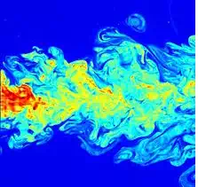
Flow visualization of a turbulent jet, made by laser-induced fluorescence. The jet exhibits a wide range of length scales, an important characteristic of turbulent flows.

Turbulence is characterized by the following features:

Irregularity 

Turbulent flows are always highly irregular. For this reason, turbulence problems are normally treated statistically rather than deterministically. Turbulent flow is chaotic. However, not all chaotic flows are turbulent.

Diffusivity 

The readily available supply of energy in turbulent flows tends to accelerate the homogenization (mixing) of fluid mixtures. The characteristic which is responsible for the enhanced mixing and increased rates of mass, momentum and energy transports in a flow is called "diffusivity".

Turbulent diffusion is usually described by a turbulent diffusion coefficient. This turbulent diffusion coefficient is defined in a phenomenological sense, by analogy with the molecular diffusivities, but it does not have a true physical meaning, being dependent on the flow conditions, and not a property of the fluid itself. In addition, the turbulent diffusivity concept assumes a constitutive relation between a turbulent flux and the gradient of a mean variable similar to the relation between flux and gradient that exists for molecular transport. In the best case, this assumption is only an approximation. Nevertheless, the turbulent diffusivity is the simplest approach for quantitative analysis of turbulent flows, and many models have been postulated to calculate it. For instance, in large bodies of water like oceans this coefficient can be found using Richardson's four-third power law and is governed by the random walk principle. In rivers and large ocean currents, the diffusion coefficient is given by variations of Elder's formula.

Rotationality 

Turbulent flows have non-zero vorticity and are characterized by a strong three-dimensional vortex generation mechanism known as vortex stretching. In fluid dynamics, they are essentially vortices subjected to stretching associated with a corresponding increase of the component of vorticity in the stretching direction—due to the conservation of angular momentum. On the other hand, vortex stretching is the core mechanism on which the turbulence energy cascade relies to establish the structure function.[clarification needed] In general, the stretching mechanism implies thinning of the vortices in the direction perpendicular to the stretching direction due to volume conservation of fluid elements. As a result, the radial length scale of the vortices decreases and the larger flow structures break down into smaller structures. The process continues until the small scale structures are small enough that their kinetic energy can be transformed by the fluid's molecular viscosity into heat. This is why turbulence is always rotational and three dimensional. For example, atmospheric cyclones are rotational but their substantially two-dimensional shapes do not allow vortex generation and so are not turbulent. On the other hand, oceanic flows are dispersive but essentially non rotational and therefore are not turbulent.

Dissipation 

To sustain turbulent flow, a persistent source of energy supply is required because turbulence dissipates rapidly as the kinetic energy is converted into internal energy by viscous shear stress. Turbulence causes the formation of eddies of many different length scales. Most of the kinetic energy of the turbulent motion is contained in the large-scale structures. The energy "cascades" from these large-scale structures to smaller scale structures by an inertial and essentially inviscid mechanism. This process continues, creating smaller and smaller structures which produces a hierarchy of eddies. Eventually this process creates structures that are small enough that molecular diffusion becomes important and viscous dissipation of energy finally takes place. The scale at which this happens is the Kolmogorov length scale.

Via this energy cascade, turbulent flow can be realized as a superposition of a spectrum of flow velocity fluctuations and eddies upon a mean flow. The eddies are loosely defined as coherent patterns of flow velocity, vorticity and pressure. Turbulent flows may be viewed as made of an entire hierarchy of eddies over a wide range of length scales and the hierarchy can be described by the energy spectrum that measures the energy in flow velocity fluctuations for each length scale (wavenumber). The scales in the energy cascade are generally uncontrollable and highly non-symmetric. Nevertheless, based on these length scales these eddies can be divided into three categories.

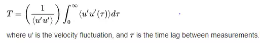
Integral time scale

The integral time scale for a Lagrangian flow can be defined as:

Integral length scales

Largest scales in the energy spectrum. These eddies obtain energy from the mean flow and also from each other. Thus, these are the energy production eddies which contain most of the energy. They have the large flow velocity fluctuation and are low in frequency. Integral scales are highly anisotropic and are defined in terms of the normalized two-point flow velocity correlations. The maximum length of these scales is constrained by the characteristic length of the apparatus. For example, the largest integral length scale of pipe flow is equal to the pipe diameter. In the case of atmospheric turbulence, this length can reach up to the order of several hundreds kilometers.: The integral length scale can be defined as

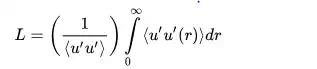
where r is the distance between 2 measurement locations, and u' is the velocity fluctuation in that same direction.

Kolmogorov length scales 

Smallest scales in the spectrum that form the viscous sub-layer range. In this range, the energy input from nonlinear interactions and the energy drain from viscous dissipation are in exact balance. The small scales have high frequency, causing turbulence to be locally isotropic and homogeneous.

Taylor microscales 

The intermediate scales between the largest and the smallest scales which make the inertial subrange. Taylor microscales are not dissipative scale but pass down the energy from the largest to the smallest without dissipation. Some literatures do not consider Taylor microscales as a characteristic length scale and consider the energy cascade to contain only the largest and smallest scales; while the latter accommodate both the inertial subrange and the viscous sublayer. Nevertheless, Taylor microscales are often used in describing the term “turbulence” more conveniently as these Taylor microscales play a dominant role in energy and momentum transfer in the wavenumber space.

Although it is possible to find some particular solutions of the Navier–Stokes equations governing fluid motion, all such solutions are unstable to finite perturbations at large Reynolds numbers. Sensitive dependence on the initial and boundary conditions makes fluid flow irregular both in time and in space so that a statistical description is needed. The Russianmathematician Andrey Kolmogorov proposed the first statistical theory of turbulence, based on the aforementioned notion of the energy cascade (an idea originally introduced by Richardson) and the concept of self-similarity. As a result, the Kolmogorov microscales were named after him. It is now known that the self-similarity is broken so the statistical description is presently modified.[10] Still, a complete description of turbulence remains one of the unsolved problems in physics.

According to an apocryphal story, Werner Heisenberg was asked what he would ask God, given the opportunity. His reply was: "When I meet God, I am going to ask him two questions: Why relativity? And why turbulence? I really believe he will have an answer for the first."  A similar witticism has been attributed to Horace Lamb (who had published a noted text book on Hydrodynamics)—his choice being quantum electrodynamics (instead of relativity) and turbulence. Lamb was quoted as saying in a speech to the British Association for the Advancement of Science, "I am an old man now, and when I die and go to heaven there are two matters on which I hope for enlightenment. One is quantum electrodynamics, and the other is the turbulent motion of fluids. And about the former I am rather optimistic." A more detailed presentation of turbulence with emphasis on high-Reynolds number flow, intended for a general readership of physicists and applied mathematicians, is found in the Scholarpedia articles by Benzi and Frisch and by Falkovich. There are many scales of meteorological motions; in this context turbulence affects small-scale motions.