Field measurements

The evaluation of surface irrigation at the field level is an important aspect of both management and design. Field measurements are necessary to characterize the irrigation system in terms of its most important parameters, to identify problems in its function, and to develop alternative means for improving the system. System characterization necessitates a series of basic field measurements before, during, and after the irrigation. The objectives of the evaluation will dictate whether the field measurements are comprehensive or are simplified for special purposes. In some cases, there are alternative methodologies and equipment for accomplishing the same ends. The selection provided herein is based on a limited selection found to be most useful during numerous field evaluations and, in some measure, the practicality in the international sense.

Five classes of field measurements are presented:

(1) field topography and configuration;

(2) water requirements;

(3) infiltration;

(4) flow measurement; and

(5) irrigation phases.

Field topography and configuration

All field evaluations should include a relatively simple assessment of the field topography and layout. These measurements are well enough known that only their brief mention is required. There is first of all the field's primary elevations. This information requires that a surveying instrument be used to measure elevations of the principal field boundaries (including dykes if present), the elevation of the water supply inlet (an invert and likely maximum water surface elevation), and the elevations of the surface and subsurface drainage system if possible. These measurements need not be comprehensive nor as formalized as one would expect for a land levelling project.  The field topography and geometry should be measured. This requires placing a simple reference grid on the field, usually by staking, and then surveying the elevations of the field surface at the grid points to establish slope and slope variations. Usually one to three lines of stakes placed 20-30 metres apart or such that 5-10 points are measured along the expected flow line will be sufficient. For example, a border or basin would require at most three stake lines, a furrow system as little as one, depending on the uniformity of the topography. The survey should establish the distance of each grid point from the field inlet as well as the field dimensions (length of the field in the primary direction of water movement as well as field width).

There are important items of information that should be available from the survey:

(1) the field slope and its uniformity in the direction of flow and normal to it;

(2) the slope and area of the field; and

(3) a reference system in the field establishing distance and elevation changes.

It is also worthwhile at this stage of the evaluation to record the location and extent of major soil types (this may require sampling and some laboratory analyses). The cropping pattern should be determined and, if a crop is on the field at the time of the evaluation, any obvious differences in growth and vigour should be noted. Similarly, the cultivation practices should be recorded.

Determining water requirements

· Evapotranspiration and drainage requirements

· Soil moisture principles

· Soil moisture measurements

· An example problem on soil moisture

The irrigation system may not be designed to supply the total amount of moisture required for crop growth. In some cases, precipitation or upward flow from a water table may contribute substantially towards fulfilling crop water requirements. It is also unrealistic to expect that irrigation can be practiced without losses due to deep percolation, or tailwater runoff. The fraction of the water that is used should be maximized, but this fraction cannot be 100 percent without other serious problems developing such as a salt build-up in the crop root zone. The dependency on irrigation in an area requires some analyses of the water balance. Water balance may have three perspectives. The first is the balance of agricultural demands within a watershed as depicted in Figure 15. The outcome of such an analysis establishes the safe yield of water from various sources and thereby indicates the area of a project, the priorities among projects, and the configuration of the large systemic components of the project. An evaluation at the field level presumes that this information is available, and it should be generally understood in as much as the limits of on-farm irrigation may be dictated by the magnitude and distribution of the total water supply.

Figure 15. The perspective of water balance at the river basin level (from Walker, 1978)

The second water balance perspective, illustrated in Figure 16, is the water balance within the farm or command area. An individual field is generally irrigated in concert with others in the command or farm through sharing the water delivered through a canal turnout or a well. Fields also typically share drainage channels. Water balance at the farm or command area level is established on a field's access to water, its priority, timing and duration. Again, a field evaluation presumes that these factors have been formulated and can be determined. Figure 17 illustrates the perspective of water balance at the field level.

Figure 16. A perspective of the on-farm water balance

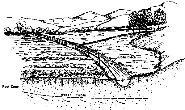
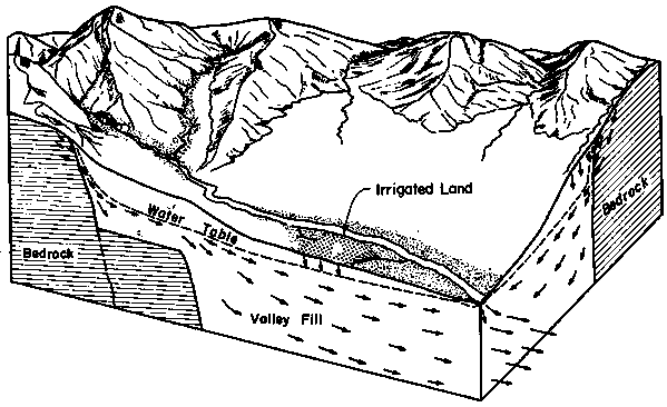
Figure 17. The perspective of water balance at the field level

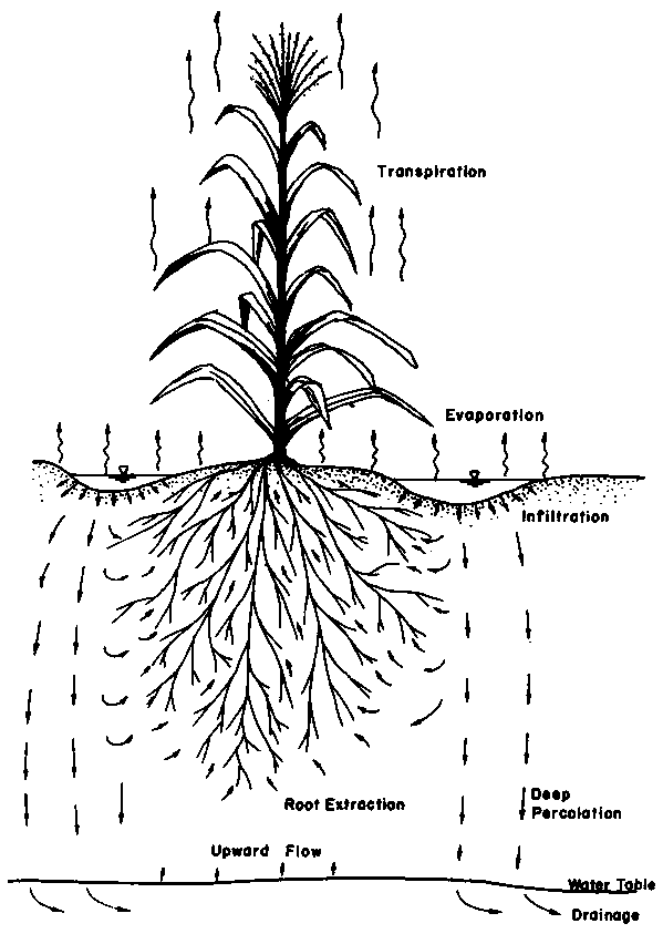
The water balance within the confines of a field is a useful concept for characterizing, evaluating or monitoring any surface irrigation system. In using this aspect of water balance, an important consideration is the time frame in which the computations are made, i.e. whether the balance will use annual data, seasonal data, or data describing a single irrigation event. If a mean annual water balance is computed, then it becomes reasonable that the change in root zone soil moisture storage could be assumed as zero. In some irrigated areas, precipitation events are so light that the net rainfall can be reasonably assumed to equal the measured precipitation. Under other circumstances, various other terms can be neglected. In fact, the time base and field conditions are often selected to eliminate as many of the parameters as possible in order to study the behaviour of single parameters. One of the more important is crop evapotranspiration. The upward movement of groundwater to the root zone can usually be ignored if the water table is at least a metre below the root zone. Then if the soil moisture is measured before and after a period when there is no precipitation or irrigation, the depletion from the root zone is a viable estimate of crop water use.

There are two particularly important components in the field water balance which impact design and evaluation. The first is the irrigation requirement of the crop, or its evapotranspiration and leaching needs. This is a design parameter and will be briefly described here, but a detailed treatment is left to the FAO Irrigation and Drainage Paper 24, Crop Water Requirements, by Doorenbos and Pruitt (FAO, 1977). The second important component deals with field evaluation and concerns the nature of moisture content changes in the soil profile.

 Evapotranspiration and drainage requirements

Evapotranspiration, ET, is dependent upon climatic conditions, crop variety and stage of growth, soil moisture depletion, and various physical and chemical properties of the soil. A two step procedure is generally followed in estimating ET: (1) the seasonal distribution of reference crop "potential evapotranspiration", E_tp, which can be computed with standard formulae; and (2) the E_tp is adjusted for crop variety and stage of growth. Other factors like moisture stress can be ignored for the purposes of design computations. There are perhaps twenty commonly used methods for calculating evapotranspiration, ranging in complexity from the Blaney-Criddle Method using primarily mean monthly temperature to more complete equations such as the Penman Method requiring radiation, temperature, wind velocity, humidity and other factors comprising the net energy balance at the crop canopy. The actual crop water demand depends on its stage of development and variety. Generally it is estimated by multiplying E_tp by a crop growth stage coefficient, k_CO. Values of k_CO have been published by Jensen (1973), Kincaid and Heermann (1974) and Doorenbos and Pruitt (FAO, 1977) for a wide range of crops grown worldwide. Some irrigation water should be applied in excess of the storage capacity of the soil to leach salts from the rooting region, although this does not have to be achieved during each irrigation event. It can usually be applied on an annual basis. As a matter of practicality, the normally occurring deep percolation under most surface irrigation systems exceeds the leaching fraction necessary for salt balance, particularly for the first and second irrigations each season when deep percolation losses are typically greatest. In addition, precipitation helps leach salts throughout the year. Nevertheless some irrigated areas maintain a salt balance in the root zone with excess leaching during only years of plentiful water supplies, which may occur as infrequently as every three to eight years.

Soil moisture principles

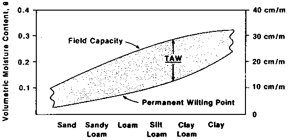
Important soil characteristics in irrigated agriculture include: (1) the water-holding or storage capacity of the soil; (2) the permeability of the soil to the flow of water and air; (3) the physical features of the soil like the organic matter content, depth, texture and structure; and (4) the soil's chemical properties such as the concentration of soluble salts, nutrients and trace elements. The total available water, TAW, for plant use in the root zone is commonly defined as the range of soil moisture held at a negative apparent pressure of 0.1 to 0.33 bar (a soil moisture level called 'field capacity') and 15 bars (called the 'permanent wilting point'). The TAW will vary from 25 cm/m for silty loams to as low as 6 cm/m for sandy soils. Some typical values of TAW, field capacity, permanent wetting point and miscellaneous features have been given in various texts. A typical summary is shown in Figure 18.

Figure 18. Relationships between soil types and total available soil moisture holding capacity, field capacity and wilting point (from Walker and Skogerboe, 1987)

Other important soil parameters include its porosity, f , its volumetric moisture content, q ; its saturation, S; its dry weight moisture fraction, W; its bulk density, g _b; and its specific weight, g _s. The relationships among these parameters are as follows.

The porosity, f , of the soil is the ratio of the total volume of void or pore space, V_p, to the total soil volume V:

f = V_p/V (1)

The volumetric water content, q , is the ratio of water volume in the soil, V_W, to the total volume, V:

q = V_b/V (2)

The saturation, S, is the portion of the pore space filled with water:

S = V_W/V_p (3)

These terms are further related as follows:

q = S * f (4)

When a sample of field soil is collected and oven-dried, the soil moisture is reported as a dry weight fraction, W:

 (5)

To convert a dry weight soil moisture fraction into volumetric moisture content, the dry weight fraction is multiplied by the bulk density, g _b; and divided by specific weight of water, g _w which can be assumed to have a value of unity. Thus:

q = g _b W/g _w (6)

The g _b is defined as the specific weight of the soil particles, g _s, multiplied by the particle volume or one-minus the porosity:

g _b = g _b * (1 - f ) (7)

The volumetric moisture contents at field capacity, q _fc, and permanent wilting point, q _wp, then are defined as follows:

q _fc = g _b W_fc/g _w (8)

q _wp = g _b W_wp/g _w (9)

where W_fc and W_wp are the dry weight moisture fractions at each point.

The total available water, TAW is the difference between field capacity and wilting point moisture contents multiplied by the depth of the root zone, RD (refer to Table 1):

TAW = (q _fc - q _wp) RD (10)

Table 1 AVERAGE ROOTING DEPTHS FOR COMMONLY GROWN CROPS ¹

Crop	Root Depth (metres)
Alfalfa	1.5
Almonds	1.8
Apricots	1.8
Artichokes	1.4
Asparagus	1.5
Bananas	0.9
Beans	0.9
Beets	0.8
Broccoli	0.5
Cabbage	0.5
Cantaloupes	1.5
Carrots	0.9
Cauliflower	0.6
Celery	0.4
Cherries	2.0
Citrus	1.4
Corn (maize)	1.3
Cotton	1.2
Cucumber	1.1
Eggplant	0.9
Figs	1.5
Grains and flax	1.2
Grapes	1.5
Groundnuts.	0.7
Ladino clover	0.6
Lettuce	0.3
Melons	1.3
Milo (Sorghum)	1.2
Mustard	1.1
Olives	1.5
Onions	0.3
Palm Trees	0.9
Peaches	1.6
Pears	1.6
Peas	0.8
Peppers	0.9
Pineapple	0.5
Potatoes	0.9
Prunes	1.5
Pumpkins	1.8
Radishes	0.5
Safflower	1.5
Soybeans	1.0
Spinach	0.6
Squash (summer)	0.9
Strawberries	0.5
Sudan grass	1.8
Tomatoes	1.5
Turnips	0.9
Walnuts	2.0
Watermelon	1.2

Summarized from Marr (1967) and Doorenbos and Pruitt (FAO, 1977)

The Soil Moisture Deficit, SMD, is a measure of soil moisture between field capacity and existing moisture content, q _i, multiplied by the root depth:

SMD = (q _fc - q _i) * RD (11)

A similar term expressing the moisture that is allotted for depletion between irrigations is the 'Management Allowed Deficit', MAD. This is the value of SMD where irrigation should be scheduled and represents the depth of water the irrigation system should apply. Later this will be referred to as Z_req indicating the 'required depth' of infiltration.

Soil moisture measurements

The soil moisture status requires periodic measurements in the field, from which one can project when the next irrigation should occur and what depth of water should be applied. Conversely, such data can indicate how much has been applied and its uniformity over the field. As noted in the previous subsections, bulk density, field capacity and the permanent wilting point are also needed.

There are numerous techniques for evaluating soil moisture. Perhaps the most useful are gravimetric sampling, the neutron probe and the touch-and-feel method.

i. Gravimetric sampling

Gravimetric sampling involves collecting a soil sample from each 15-30 cm of the soil profile to a depth at least that of the root penetration. Typical samplers are shown in Figure 19. The soil sample of approximately 100-200 grammes is placed in an air tight container of known weight (tare) and then weighed. The sample is then placed in an oven heated to 105° C for 24 hours with the container cover removed. After drying, the soil and container are again weighed and the weight of water determined as the before and after readings. The dry weight fraction of each sample can be calculated using Eq. 5. Knowing the bulk density, one can determine moisture contents from Eq. 6 and the soil moisture depletion from Eq. 11.

Figure 19. Small equipment used for collecting soil samples from the field

a. sampling auger

b. sampling tube

ii. The neutron Probe

The neutron probe and scaler for making soil moisture measurements are illustrated in Figure 20. The neutron probe is inserted at various depths into an access tube and the count rate is read from the scaler. The manufacturers of neutron probe equipment furnish a calibration relating the count rate to volumetric soil moisture content. Field experience suggests that these calibrations are not always accurate under a broad range of conditions so it is advisable for the investigator to develop an individual calibration for each field or soil type. Most calibration curves are linear, best fit lines of gravimetric data and scaler readings but may in some cases be slightly curvilinear (van Baval et al., 1963).

Figure 20. A neutron probe and scaler for soil moisture measurements (after Walker and Skogerboe, 1987)

The volume of soil actually monitored in readings by the neutron probe depends on the moisture content of the soil, increasing as the soil moisture decreases. The accuracy of soil moisture determinations near the ground surface is affected by a loss of neutrons into the atmosphere thereby influencing measurements prior to an irrigation more than afterwards. As a consequence, soil moisture measurements with a neutron probe are usually unreliable within 10-30 cm of the ground surface.

iii. Touch-and-feel

As a means of developing a rough estimate of soil moisture, the Touch-and-feel method can be used. A handful of soil is squeezed into a ball. Then the appearance of the squeezed soil can be compared subjectively to the descriptions listed in Table 2 to arrive at the estimated depletion level. Merriam (1960) has developed a similar table which gives the moisture deficiency in depth of water per unit depth of soil. Over the years various investigators have compared actual gravimetric sample results to the Touch-and-Feel estimates, finding a great deal of error depending on the experience of the sampler.

Table 2 GUIDELINES FOR EVALUATING SOIL MOISTURE BY FEEL

Percent	Feel or Appearance of Soil
Depletion	Loamysands to fine sandy loams	Fine sandy loams to silt loams				Silt loams to clay loam
0 (field capacity)	no free water on ball* but wet outline on hand				Same			same
0-25	makes ball but breaks easily and does not feel slick				makes tight ball, ribbons easily, slightly sticky and slick			easily ribbons slick feeling
25-50	balls with pressure but easily breaks			pliable ball, not sticky or slick, ribbons and feels damp			pliable ball, ribbons easily slightly slick
50-75	will not ball, feels dry			balls under pressure but is powdery and easily breaks			slightly balls still pliable
75-100	dry, loose, flows through fingers		powdery, dry, crumbles						hard, baked, cracked, crust

* A "Ball" is formed by squeezing a soil sample firmly in one's hand
A "Ribbon" is formed by squeezing soil between one's thumb and forefinger.

iv. Bulk density

Measurements of bulk density are commonly made by carefully collecting a soil sample of known volume and then drying the sample in an oven to determine the dry weight fraction. Then the dry weight of the soil, W_b is divided by the known sample volume, V, to determine bulk density, g _b:

g _b = W_b V (12)

Most methods developed for determining bulk density use a metal cylinder sampler that is driven into the soil at a desired depth in the profile. Bulk density varies considerably with depth and over an irrigated field. Thus, it is generally necessary to repeat the measurements in different places to develop reliable estimates.

v. Field capacity

The most common method of determining field capacity in the laboratory uses a pressure plate to apply a suction of -1/3 atmosphere to a saturated soil sample. When water is no longer leaving the soil sample, the soil moisture in the sample is determined gravimetrically and equated to field capacity.

A field technique for finding field capacity involves irrigating a test plot until the soil profile is saturated to a depth of about one metre. Then the plot is covered to prevent evaporation. The soil moisture is measured each 24 hours until the changes are very small, at which point the soil moisture content is the estimate of field capacity.

vi. Permanent wilting point

Generally, at the permanent wilting point the soil moisture coefficient is defined as the moisture content corresponding to a pressure of -15 atmospheres from a pressure plate test. Although actual wilting points can be somewhere between -10 and -20 atm, the soil moisture content varies little in this range. Thus, the -15 atm moisture content provides a reasonable estimate of the wilting point.

An example problem on soil moisture

A cylindrical soil sample 10 cm in diameter and 10 cm long has been carefully taken so that negligible compaction has occurred. It was weighed before oven drying (1284 grammes) and after (1151 g). What soil parameters can be identified?

1. Bulk Density:

g _b = W_b / V (12)

= 1151 g / [(3.14 * (10 cm)²/4) * 10 cm] = 1.466 g/cm³

2. Dry Weight Moisture Fraction:

 (5)

= (1284 g / 1151 g) / 1151 g = 0.116

3. Volumetric Moisture Content:

= (1.466 g / 1..0 g/cm³) * 0.116 = 0.170 (6)

4. Water Content Expressed as a Depth:

Depth of Water = q * Depth of Soil

= 0.17 cm of water per cm of soil.

Now suppose the soil sample is carefully rewetted to the saturation point, utilizing 314 9 of water to do so. What other soil properties are identified?

5. Porosity:

f = V_p / V (1)

= = 0.40

6. Initial Soil Saturation:

S = q / f = 0.170 / 0.40 = 0.425 (4)

7. Specific Weight of the Soil Particles:

g _S = g _b / (1 - f ) = 1.466 / 0.60 = 2.44 g/cm³ (7)

Finally, suppose the sample is allowed to drain under conditions where it does not dry due to evaporation until the water in the sample is under a negative pressure of -1/3 atm so that one can assume it is at field capacity. The water draining from the sample was collected and weighed 160 g. What other evaluations are now possible?

8. Field Capacity Volumetric Moisture Content:

q _fc = g _b W_fc / g _w (8)

9. Soil Moisture Depletion at the Time of Sampling:

SMD = (q _fc - q _i)* RD = (0.196 - 0.170) RD = 0.026 RD (11)

If the root depth is 100 cm,

SMD = 2.6 cm

 Infiltration

· Infiltration functions

·  Typical infiltration relationships

·  Measuring infiltration

·  An example infiltrometer test

Infiltration is the most important process in surface irrigation. It essentially controls the amount of water entering the soil reservoir, as well as the advance and recession of the overland flow. Typical curves of infiltration rate, I, and cumulative infiltration, Z, are shown in Figure 21. Irrigation of initially dry soil exhibits an infiltration rate with a high initial value which decreases with time until it becomes fairly steady, which is termed the 'basic infiltration rate'. Infiltration is a complex process that depends upon physical and hydraulic properties of the soil moisture content, previous wetting history, structural changes in the layers and air entrapment.

Figure 21. Typical infiltration rate and cumulative infiltration function

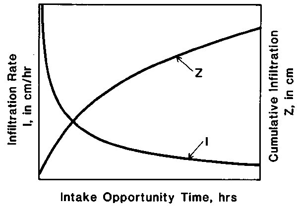
In surface irrigation, infiltration changes dramatically throughout the irrigation season. The water movements alter the surface structure and geometry which in turn affect infiltration rates. The term 'intake' is often used interchangeably with 'infiltration', particularly where the geometry of the field influences the infiltration process.

 Infiltration functions

Both the procedures for interpreting field data and those covering surface irrigation design require that infiltration be described mathematically. There are a number of mathematical equations to choose from, probably none as versatile as the two so-called Kostiakov-Lewis relationships.

The simplest approximation of cumulative infiltration is written:

Z = k r^a (13)

in which,

Z = cumulative infiltration in units of volume per unit length per unit width;
r = intake opportunity time; and
k and a = empirical constants.

Equation 13 is simple, easy to define, and widely used. Its major disadvantage is its inadequacy in describing infiltration over long time periods. The infiltration rate based on Eq. 13 is:

I = a k r^a-1 (14)

Since a is always less than unity, I approaches zero at infinite time. This is a condition not typically encountered in the field. Some soils do, however, have extremely small infiltration rates after a period of time and Eqs. 13 and 14 can be used effectively.

A more general infiltration function is the extended form of Eq. 13:

Z = k r^a + f_o r (15)

in which f_o is the long term steady, or 'basic' infiltration rate in units of volume per unit length per unit time and width. Equation 15 easily reduces to Eq. 13 if the soil intake rate at long times approaches a zero value or if the irrigation event is short compared to the time required for the infiltration to reach a steady rate. Equation 15 gives a better long term approximation on many soils. One case in particular where Equation 15 has been shown superior to Eq. 13 is when estimates of field runoff are being made.

The infiltration rate using Eq. 15 is:

I = a k r^a-1 + f_o (16)

Typical infiltration relationships

The Soil Conservation Service of the US Department of Agriculture developed a series of 'intake families' to assist field technicians and engineers. The curves were based on field measurements made over a period of years at numerous locations. They are given in the SCS National Engineering Handbook, Chapters 4 and 5 dealing with border and furrow irrigation. To be consistent with the analysis contained in this guide, a number of modifications were made to the SCS intake family concept. First, the curves were redefined in the format of Eq. 15 by defining a basic intake rate, f_o, for each family, and then recomputing the values of a and k. Figure 22 shows the intake curves which result (Gharbi, 1984). Table 3 gives the k, a, and f_o coefficients for each intake curve along with the typical soil type. The units employed are m³/m of length per 'characteristic' width of the field. For borders and basins, the 'characteristic' width is l metre. For furrows it is the wetted perimeter of the furrow cross-sections. Thus, to use the functions for furrow irrigation, it is necessary to estimate the wetted perimeter for the inlet discharge, divide this value by the furrow to furrow spacing, and then adjust the k and f_o values by multiplying each by the resulting perimeter to spacing ratio. The k and f_o values should not be reduced below 50 percent as would be the case for widely spaced furrows.

Figure 22. Kostiakov-Lewis intake relationships based on the US Dept. of Agriculture's intake series

Table 3 KOSTIAKOV-LEWIS INTAKE PARAMETERS (after Gharbi, 1984)

curve no.	k m/min^a	a	fo m/min	ave. 6 hr intake rate	soil type
.05	.00426	.258	.000022	2	Clay
.10	.00383	.317	.000035	4
.15	.00360	.357	.000046	5
.20	.00346	.388	.000057	6	clay loam
.25	.00337	.415	.000068	7
.30	.00330	.437	.000078	8
.35	.00326	.457	.000088	9
.40	.00323	.474	.000098	10
.45	.00321	.490	.000107	12	silty loam
.50	.00320	.504	.000117	13
.60	.00320	.529	.000136	15
.70	.00321	.550	.000155	17
.80	.00324	.568	.000174	20
.90	.00328	.584	.000193	22	sandy loam
1.00	.00332	.598	.000212	25
1.50	.00361	.642	.000280	35	Sandy
2.00	.00393	.672	.000339	45

The segregation of the intake families by soil type is qualitative, but it serves the field technician or irrigation engineer during preliminary design or evaluation work. The relationships given in Figure 22 and Table 3 are not intended as substitutes for field measurements when they can be made. These measurements are among the most important tasks that should be undertaken as part of surface irrigation work.

 Measuring infiltration

Infiltration is one of the most difficult parameters to define accurately. The importance of infiltration combined with the difficulties in obtaining reliable data suggests that the field technician should expect to spend considerable time evaluating infiltration. The irrigation engineer should ensure that infiltration has been adequately defined. Four commonly employed techniques for measuring infiltration are noted here.

 These are

(1) cylinder infiltrometers;

(2) ponding;

(3) blocked recirculating infiltrometers; and

(4) a deduction of infiltration from evaluation of the advance phase and the tailwater hydrograph.

i. Cylinder infiltrometers

Haise et al. (1956) presents one of the most complete instructions on the use of cylinder infiltrometers. A metal cylinder (Figure 23) with a diameter of 30 cm or more and a height of about 40 cm is driven into the soil, using a driving plate set on top of the infiltrometer and a heavy hammer.

Figure 23. A schematic of a ring infiltrometer and driving plate (after Haise et al., 1956)

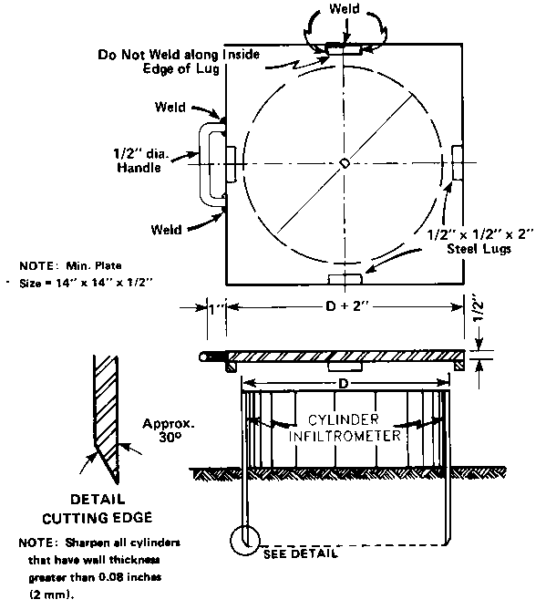
The procedure for installing the cylinder infiltrometers is to begin by examining and selecting possible sites carefully for signs of unusual surface disturbance, animal burrows, stones that might damage the cylinder, etc. Areas that may have been affected by unusual animal or machinery traffic should be avoided. The individual cylinders used for a single test should be set within a 0.2 ha area so that they can conveniently be run simultaneously. Then the cylinder is set in place and pressed firmly into the soil, after which the driving plate is placed over the cylinder and tampered with the driving hammer until the cylinder is driven to a depth of about 15 cm. The cylinder should be driven so that the driving plate is maintained in a level plane which will require that it be checked frequently to keep it properly oriented.

It is generally suggested that a buffer ring around the infiltrometer be installed so that water infiltrating from the infiltrometer will percolate vertically and thereby preserve the integrity of the measurement. There have been, however, a large number of comparisons between buffered and non-buffered readings and generally one concludes that the spatial variability in the field is so much larger than the effect of buffering that it is not worthwhile to add the substantial effort of installing and operating the buffer. In addition, most comparisons cannot detect the effect of the buffer. Given the accuracy of the method in depicting representative infiltration, any error caused by omitting the buffer is insignificant. Thus, the buffered cylinder infiltrometer testing is not recommended in this guide.

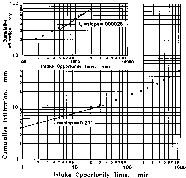
After the infiltrometer has been installed, the test is conducted in the following manner. The volume of the cylinder above the soil is carefully measured (diameter, depth, etc.). A gauge of almost any type is fixed to the inner wall so that the water level changes that occur can be measured. A pre-measured volume, about 80-90 percent of the infiltrometer capacity of water similar to the irrigation water, is added quickly to the infiltrometer. When the water surface is quieted, an initial reading should be taken. The infiltration that occurs during the period between the start of the test and this first measurement is the difference between the computed initial level and the first actual reading:

 (17)

Additional measurements should be recorded at periodic intervals, 5 to 10 minutes at the start of the tests, expanding to 30 to 60 minute intervals after 3 or 4 readings, but the observation frequencies should be adjusted to infiltration rates (see Figure 24 for a convenient recording form). Measurements should be continued until the intake rates are constant over a 1 to 2 hour period.

Figure 24. Data recording form for ring infiltrometer tests (after Haise et al., 1956)

When the water level has dropped about one-half of the depth of the cylinder, water should be added to return the surface to its approximate initial elevation. The depth should be maintained in the cylinder between 6 and 10 cm throughout the test. When water is added, it is necessary to record the level before and after filling. The interval between these two readings should be as short as possible to avoid errors due to infiltration during the refilling period.

Where the infiltration rate indicated by a single cylinder is unusually high, there is a possibility that either the cylinder has been improperly installed or it has been installed over a crack or root tube in the soil. These possibilities should be checked at the conclusion of a test.

Analysis of the data is usually made by plotting the data on logarithmic paper (cumulative depth, Z, on the vertical axis, cumulative time, t, on the horizontal axis). If the test is run long enough to establish a steady infiltration rate, as it should be approximately, this plot will not be linear. To evaluate the infiltration function, select readings near the later part of the test and take the slope as the basic intake rate, f_o. Then use the slope of the first few data points on the logarithmic paper to define the slope, a. The intercept of the horizontal axis at 1.0 is the k value. This procedure assumes that at short times the contribution to cumulative infiltration from the steady state, f_o term in Eq. 15 is negligible. These assumptions are better for the heavy soils than for the light soils.

ii. Ponding methods

Ponds can be created using bunds or dykes around an area on the ground surface and operated in the same manner and by using the same procedures discussed above for cylinders. The ponding; method can be used in small basins and other larger ground surface areas to evaluate the infiltration rates of a larger fraction of the field. The disadvantage of this technique is that edge effects can be significant. This problem can be overcome by giving special care to the sealing of the pond perimeter with compacted clay or installing a plastic barrier. The operational and data gathering procedures, including the forms for recording data, are the same as for cylinder infiltrometers. The application of the ponding; technique to furrows requires a slightly different infiltrometer configuration. The total infiltration in a furrow consists of water moving laterally through the furrow sides as well as vertically downward. Bondurant (1957) developed a 'blocked' furrow infiltrometer which recognizes this special feature of furrows. Two sharp edged plates are driven into both ends of a furrow section to isolate a short length. The furrow geometry is then determined (as will be discussed later in this section) so the depth of water can be determined at time zero. Again, a known volume of water is added to the test section and readings begin. Since the furrow cross-sectional area declines with depth, it is best to maintain a fixed water level and record the water necessary to do so as shown in Figure 25. For the data analyses, the reservoir readings need to be adjusted for the difference in surface area between the furrow section and the reservoir, i.e. the reservoir readings of cumulative infiltration need to be multiplied by the ratio of the furrow surface area to the reservoir cross-sectional area. The remainder of the data analysis is the same.

Figure 25. Blocked furrow infiltrometer (after Walker and Skogerboe, 1987)

The issue of using buffer furrows must be considered. Where buffering is not considered important in cylinder or pond infiltration measurements, it can be important in furrow cases. Judgement must be exercised on this point. For silt and clay soils, the basic intake rate will generally be reached before the wetting fronts of adjacent furrows meet in the soil between furrows and the buffering is probably not necessary. In sandy soils, this may not be the case so the basic intake rate may be influenced by the soil moisture distribution after the wetting fronts meet. Thus, the buffering would be necessary to determine accurate readings.

iii. Recycling infiltrometers

Another innovation for evaluating infiltration, primarily in furrows is the recycling infiltrometer. The advantage of this technique is that both the geometric and hydraulic conditions encountered during irrigation are simulated during the test. This provides a better approximation of actual field situations than the static methods described above. The dynamic changes in soil-water interface must be realistically simulated. The movement of suspended particles develops a different surface condition than under the static water surface. The static case tends to form a more impermeable soil layer than would occur under usual conditions of overland flow. The recycling infiltrometer for furrows is shown in Figure 26. A sump is installed at each end of a furrow section 5 to 6 metres in length. The sumps should be carefully buried in the ground so that the sump inverts correspond with the furrow bed elevation. Water is pumped from the water supply reservoir via a hose into the furrow inflow sump. It then advances across the furrow test section and is collected in the tailwater sump. Another pump then moves the water back into the water supply reservoir. The discharge in the system can be regulated by various valves to maintain a constant water level in the tailwater sump.

Figure 26. Recycling furrow infiltrometer (after Malano, 1982)

a. recycling furrow test section

b. supply reservoir

c. tailwater sump and pumpback system

d. recording pressure sensor on supply reservoir

As with the blocked furrow technique, the furrow cross-section must be measured so that the relationship of the surface area to that of the reservoir is known. Thus, the cumulative infiltration function is developed in the same way it is for cylinder and pond measurements, i.e. the cumulative infiltration is the reservoir readings corrected by the ratio of surface areas in the furrow and the reservoir.

The time required to complete the advance phase can be minimized by increasing the furrow inflow discharge rate for a few minutes. The decline in the reservoir volume is a direct reading of the cumulative infiltration into the furrow.

 An example infiltrometer test

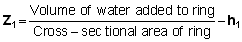
Table 4 gives one set of cylinder infiltrometer data taken from a field study. A plot of cumulative depth versus cumulative time is given in Figure 27.

Figure 27. Plot of cumulative time and infiltration for the example problem

From the last four readings, a linear slope of the plot is calculated as follows:

time	Z	D Z	t	fo	fo
(min)	(mm)			mm/min	m/min
960	50
		6	180	0.033	0.000033
1140	56
		5	180	0.028	0.000028
1320	61
		4	160	0.025	0.000025
480	65

Table 4 EXAMPLE CYLINDER INFILTROMETER DATA

Time Readings		Gauge Readings
Clock	Cumulative	Gauge	Cumulative
hrs	min	mm	mm
0800	0	187	0
0801	1	183	4
0802	2	182	5
0804	4	181	6
0806	6	180	7
0810	10	179	8
0820	20	177	10
0830	30	176	11
0900	60	173	14
1000	120	169	18
1100	180	166	21
1200	240	163	24
1400	360	158	29
1600	480	153	34
1800	600	149	38
2400	960	137	50
0300	1140	131	56
0600	1320	126	61
0840	1480	122	65

One can see that the linear slope is changing with time even after more than 24 hours and thus the contribution to Z from the nonlinear portion is still evident. Nevertheless, these are the data available and f_o can be selected as 0.000025 m/min or .000025 m³/min per unit width per unit length. This value can be expected to be slightly higher than in reality due to the problem noted above, but the error is not large.

Now the non-linear term in Eq. 15 can be determined by examining the first points of the data. Since f_o is now estimated, an adjustment can be made as follows:

time	Z	Z-fo r
min	mm	mm
0	0	0
1	4	3.975
2	5	4.95
4	6	5.90
6	7	6.85
10	8	7.75
20	10	9.50

A regression can be run through the Z-f_o r versus t data to arrive at a and k values. k is read directly from the table as 3.975 mm/mm^a or 0.003975 m³/min^a/unit width/unit length. The value of a is found by fitting the end points:

log(9.50) = a log (20)
log(3.975) = a log (1)

and by simultaneous solution:

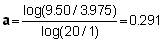
Thus,

Z = 0.003975 r ^.291 + 0.000025 r