RANS Modelling of Turbulence in Combustors
Abstract
Turbulence modelling is a major issue, affecting the precision of current numerical simulations, particularly for reacting flows. The RANS (Reynolds‐averaged Navier‐Stokes) modelling of turbulence is necessary in the development of advanced combustion systems in the foreseeable future. Therefore, it is important to understand advantages and limitations of these models. In this chapter, six widely used RANS turbulence models are discussed and validated against a comprehensive experimental database from a model combustor. The results indicate that all six models can catch the flow features; however, various degrees of agreement with the experimental data are found. The Reynolds stress model (RSM) gives the best performance, and the Rk‐ε model can provide similar predictions as those from the RSM. The Reynolds analogy used in almost all turbulent reacting flow simulations is also assessed in this chapter and validated against the experimental data. It is found that the turbulent Prandtl/Schmidt number has a significant effect on the temperature field in the combustor. In contrast, its effect on the velocity field is insignificant in the range considered (0.2–0.85). For the present configuration and operating conditions, the optimal turbulent Prandtl/Schmidt number is 0.5, lower than the traditionally used value of 0.6–0.85.
Introduction
Turbulence is one of the principal unsolved problems in physics today and its modelling is one of the major issues that affect the precision of current numerical simulations in engineering applications, particularly for reacting flows. Turbulence is characterized by irregularity or randomness, diffusion, vortices and viscous dissipation, and involves a wide range of time and length scales. Despite the rapid development of computing power, large eddy simulations are limited to benchmark cases with relatively simple geometries, while direct numerical simulations of turbulent flows remain practical only at low Reynolds numbers. It is particularly true for turbulent reacting flows. Even without turbulence, combustion is a complicated process and can consist of hundreds of species and thousands of element reactions, where numerical difficulties occur [5]. Consequently, it is necessary to utilize turbulence models for the development of advanced combustion systems in the foreseeable future.
Much effort has been made to the development of turbulence modelling in the last six decades. Advances focused on constant density flows have been reviewed or described by a number of researchers and brought up to date for the second momentum closure in reacting flows. Various algebraic, one‐ and two‐equation turbulence models were systematically evaluated against a number of well‐documented non‐reacting flows, including free‐shear, boundary‐layer and separated flows. Some guidelines regarding applications of these models were provided. Recently, six eddy‐viscosity and two variants of Reynolds stress turbulence models were used to study the flow field around a ship hull. It was found that the two Reynolds stress models were able to reproduce all the salient features and the predicted Reynolds stresses and turbulence kinetic energy were in good agreement with the experimental results. Despite the considerable progresse in turbulence modelling, no universal turbulence model is available for all flows at the current time. Therefore, it is important to understand advantages and shortcomings of these models and select the best one for defined engineering problems.
In contrast to turbulence momentum transfer modelling, studies on turbulence scalar transfer modelling are limited, but are of great engineering interest. From the 1970s (CFD pioneer work) up to present, in almost all turbulent reacting flow simulations, the Reynolds analogy concept has been used to model turbulence scalar transfers (mixture fraction, species and energy or temperature). In this approach, the turbulent Prandtl (Prt) and Schmidt (Sct) numbers are used to link the turbulence scalar transfers to the momentum transfer that is calculated by a selected turbulence model. The main advantage of this approach is that the turbulence scalar transfers can be effectively computed from the modelled momentum transfer without solving a full‐second moment closure for both momentum and scalar transportations.
The Reynolds analogy concept was first postulated over a century ago on the similarity between wall shear and heat flux in boundary layers. This original hypothesis has been considerably amended and applied to general 3D (three‐dimensional) turbulent heat and species transfers. Recently, its applications to high‐Mach‐number boundary layers, turbine flows and film cooling have been studied.
In most turbulent reacting or mixing flow simulations, it has become a common practice to set Prt = Sct. Traditionally, a constant value of Prt = Sct = 0.6–0.85 has been used in jet and gas turbine flows, and these values are consistent with numerous measurements performed in the 1930s–1980s. However, low Prt and Sct numbers from 0.20 to 0.5 have been used by a large number of authors for simulating gas turbine combustors. Effort was made to validate a two‐dimensional finite difference code against a number of isothermal and reacting flow measurements, and a value of Prt = Sct = 0.5 was recommended for recirculation zone simulations. The numerical results of five RQL (rich burn, quick quench and lean burn) low‐emission combustor designs were calibrated against CARS (coherent anti‐Stokes Raman spectroscopy) temperature measurements, and good agreement was found by using Prt = Sct = 0.2. An entire combustor from the compressor diffuser exit to the turbine inlet was successfully studied, and a low value of 0.25 was used for Prt and Sct since it consistently demonstrated better agreement with the fuel/air mixing results. Moreover, the turbulence scalar mixing of a gaseous jet issued into a cross airflow was investigated, and in comparison with the available experimental data, Prt = Sct = 0.2 was recommended. The above examples suggest that for reacting flow modelling, the scalar transfer modelling or Reynolds analogy has to be investigated.
Although there are a large number of publications on numerical simulations of practical combustion systems], systematic assessment and validation of turbulence models in combustor flow fields against well‐defined comprehensive experimental results are rare.
This chapter focuses on most widely used turbulence models in practical engineering, that is RANS (Reynolds‐averaged Navier‐Stokes) models, including the Reynolds stress model (RSM), a second moment closure and five popular two‐equation eddy‐viscosity models, the standard k‐ε, renormalization group (RNG) k‐ε, realizable k‐ε (Rk‐ε), standard k‐ω and shear‐stress transport (SST) k‐ω model. The contents are based on the author’s experience and publications accumulated over many years on turbulent reacting flow studies, related to gas turbine combustion systems.
A benchmark case, a model combustor, is used as technology demonstration. Although the model combustor geometry is simple, the complex phenomena, such as jet flows, wall boundary layers, shear layers, flow separations and reattachments, as well as recirculation zones, are involved, which are fundamental features in practical combustion systems. In addition, because the model combustor geometry is much simpler than practical combustors, its boundary conditions can be well defined. More importantly, a comprehensive experimental database is available, and then the assessment of the above issues is appropriate.
In the following sections, firstly, the governing equations, turbulence models and Reynolds analogy are discussed and then the other physical models and experimental measurements are briefly described, followed by the benchmark results. Finally, a few conclusions are highlighted.
Governing equations, turbulence models and Reynolds analogy
GOVERNING EQUATIONS
The first‐moment Favre‐averaged conservation equations for mass, momentum, species, mixture fraction and total enthalpy may be expressed in a coordinate‐free form as
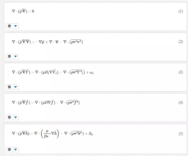
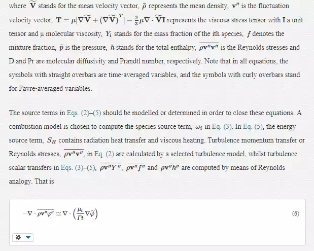
where φ stands for species, mixture fraction or enthalpy, µt is the turbulence viscosity that is computed from the chosen turbulence model and Γt represents the turbulence Prandtl (Prt) or Schmidt (Sct) number. Note that in Eq. (6), the turbulence scalar transfer coefficients, µt/Гt, are simply the products of the turbulence momentum transfer coefficient (µt) and 1/Гt.
TURBULENCE MODELS
The main features of these turbulence models are outlined here, and detailed description and formation of each model can be found in the references mentioned below. The Boussinesq hypothesis is utilized to model Reynolds stresses for the five two‐equation eddy‐viscosity turbulence models,
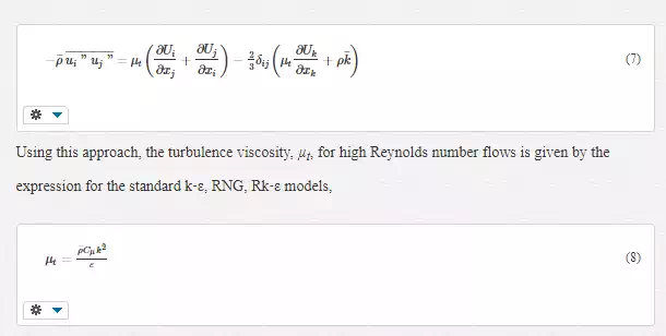
where Cµ is a constant and the values of turbulence kinetic energy, k, and dissipation rate, ε, are calculated from a pair of transport differential equations. The detailed description of the standard k‐ε turbulence model is given, which represents a pioneer work in turbulence modelling.
The RNG turbulence model is originated from a re‐normalization group theory. The major difference between the standard k‐ε and RNG models is that the coefficient of the destruction term in the turbulence dissipation rate equation is not a constant, but a function of flow mean strain rate and turbulence parameters of k and ε. Moreover, an analytical formula to account for variations of turbulent Prandtl and Schmidt numbers for the energy and species equations is provided. These modifications have made this model more responsive to the effects of strain rate and streamline curvature than the standard k‐ε model. Using this model, good agreement between the numerical and experimental results is observed for the isothermal flow over a backward facing step.
The main improvement of the Rk‐ε turbulence model is that Reynolds stresses comply with physics. That is, turbulence normal stresses always remain positive and shear stresses obey Schwarz inequality. In addition, instead of a constant, Cµ in Eq. (8) is a function of the turbulence parameters and mean strain and rotation rates. The turbulence dissipation rate equation is obtained from the dynamic equation of the mean‐square vorticity fluctuation at high Reynolds numbers. Some advantages have been observed with this model for flows with separations and recirculation zones, as well as jet spread rates over the standard k‐ε model.
The details of the standard k‐ω and SST models are given. The corresponding turbulence viscosity for high Reynolds number flows is obtained by the following two expressions, respectively,
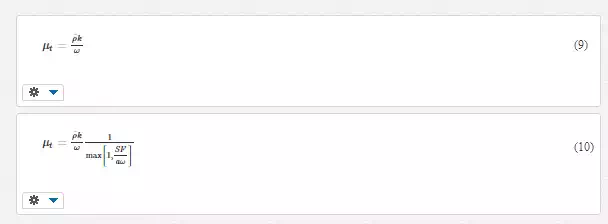
In Eqs. (9) and, a pair of transportation differential equations is used to obtain turbulence kinetic energy, k, and specific dissipation rate, ω; F equals zero in the free‐shear layer and one in the near‐wall region; ‘a' is a constant and S stands for the strain rate magnitude.
For the above two‐equation models, the linear relationship of Reynolds stresses with mean strain rate and isotropic eddy viscosity is presumed, as implied in Eqs. (7)–(10). For turbulent flow simulations with the RSM, a transportation differential equation is solved for each Reynolds stress component in the flow field. Therefore, it is expected that this second‐moment closure model is more ‘applicable’ than the two‐equation, eddy‐viscosity models. To convert Reynolds stress equations into a closed set of equations, unknown terms must be modelled by mean flow variables and/or Reynolds stresses.
REYNOLDS ANALOGY
By reducing the three‐dimensional conservation equations (2)–(5) to two‐dimensional steady boundary flows and neglecting the streamwise pressure gradient, molecular viscous terms and source terms, Eqs. (11) and (12) are obtained and the rationale and limitation of Reynolds analogy can be revealed.
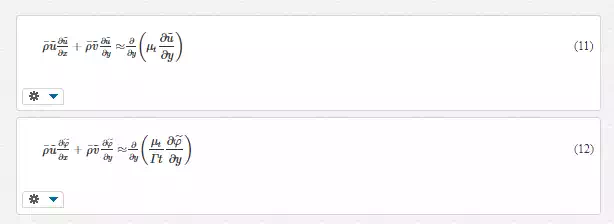
In Eqs. (11) and (12), the turbulence viscosity concept is applied to both streamwise momentum and scalar transfers. With Гt = 1, the two equations become identical. That is, under appropriate boundary conditions, the solution of all these flow parameters can be obtained from a single‐partial differential equation or the momentum and scalar fields are similar. For wall boundary flows, the original form of Reynolds analogy can be deduced [15],

The above analysis suggests that the Reynolds analogy method can be used to adequately calculate turbulence scalar transfers in a boundary type of flows, such as free jets, wall boundary layers and shear layers, where the effects of the streamwise pressure gradient, viscous and source terms are minor. However, it should be cautious to apply it to general complex three‐dimensional flows. Its failure to disturbed turbulent boundary flows has been reported by a number of authors
OTHER PHYSICAL MODELS AND NUMERICAL METHODS
For combustion modelling, the laminar flamelet, probability density function (PDF) and eddy‐dissipation (EDS) models were considered. The previous benchmark study on combustion models indicated that for mixing‐control dominated diffusion flames the temperature and velocity fields could be fairly well captured by these three combustion models.
A major advantage of the flamelet model over the probability density function and eddy‐dissipation models is that detailed more realistic chemical kinetics can be incorporated into turbulent reacting flows. For the present case, the propane‐air chemical mechanism was used. This mechanism was consisted of 228 element reactions, and 31 chemical species, i.e. O2, N2, CO2, H2O, C3H8, CH4, H2, CHO, CH2O, CH2CO, CH3CO, CH3CHO, C2H, C2H2, C2H3, C2H4, C2H5, C2H6, C3H6, O, OH, H, H2O2, HO2, CO, CH, CH2, CH3, C2HO, N*C3H7 and I*C3H7.
The PDF combustion model is based on the mixture fraction approach with an assumption of fast chemistry. It offers some advantages over the EDS or EDS‐finite‐rate models and allows intermediate (radical) species prediction, more thorough turbulence‐chemistry coupling and dissociation effect. Eighteen species were considered for the PDF model, including C3H8, CO2, H2O, O2, N2, CO, HO, H, O, H2, C3H6, C2H6, C2H4, CH4, CH3, CH2, CH and C(s). The selection of these species was based on the basic chemical kinetics and requirements for pollutant predictions. As full chemical equilibrium gave considerable errors in temperature on the rich side of hydrocarbon flames, to avoid this, a partial equilibrium approach was applied in the rich flame region. When the instantaneous equivalence ratio exceeded 1.75, the combustion reaction was considered extinguished and unburned fuel coexisted with reacted products.
The EDS model is widely accepted in diffusion flame modelling. For this model, the reaction rate is governed by turbulent mixing, or the large‐eddy mixing timescale, k/ε. In the present case, the heat radiation from the hot gas mixture to the surroundings was computed by the discrete ordinates model, where the local species mass fractions were used to calculate the absorption coefficient of gaseous mixture in the flow. At all wall boundaries, an enhanced wall boundary approach was utilized, where the traditional two‐layer zonal model was improved by smoothly combining the viscous sub‐layer with the fully turbulent region.
The specific heat of species was calculated by polynomials as a function of temperature. For the case of the flamelet and PDF models, the polynomials were determined from the JANAF tables; while in the case of the EDS model, the polynomials from Rose and Cooper were used, where the chemical dissociation was considered. For other thermal properties such as molecular viscosity, thermal conductivity and diffusivity, the values of air at 900 K were used.
A segregated solver with a second‐order‐accuracy scheme from a commercial software, Fluent, was used to resolve the flow fields. The results were well‐converged, and the normalized residuals of the flow variables were about or less than 10–5 for all test cases. The axial velocities monitored in shear layers of the flow fields were unchanged for the first four digits. A LINUX cluster with eight nodes and 64‐GB RAM/node was employed to perform all numerical simulations.
Benchmark experimental measurements
A series of experimental measurements on a diffusion flame model combustor were carried out at the National Research Council of Canada (NRCC). The results provided a comprehensive database for the evaluation and development of various physical models, including mean and fluctuation velocity components, mean temperature, wall temperature, radiation heat flux through walls, as well as species concentrations.
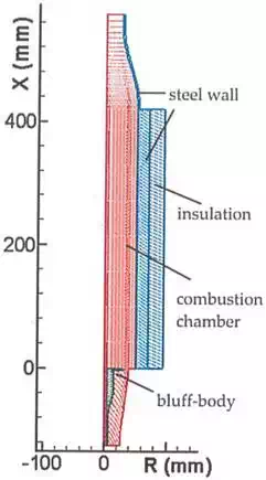
The test apparatus and model combustor are shown in Figure 1 where all dimensions are in mm. The model combustor consists of the air and fuel inlet section, combustion chamber and contracted exhaust section. Fuel entered the combustion chamber through the centre of the bluff body, while air flowed into the chamber around a disc flame‐holder. The combustor was mounted on a three‐axis traversing unit with a resolution of ±100 µm. Fuel was commercial grade propane, and air was from a dry air supply. Both air and fuel flow rates were regulated by Sierra Side‐Trak mass‐flow controllers with 2% accuracy of the full scale (100 l/min for fuel and 2550 l/min for air).
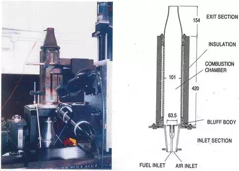
FIGURE 1.
The test apparatus and model combustor.
A 25.4‐mm thick fibre blanket of Al2O3 was wrapped around the combustion chamber in order to reduce the heat losses through the combustor walls. The optical and physical access to the combustion chamber was through four windows. The viewing area of the windows measured 17 mm in width, 342 mm in length and 44–388 mm from the disk flame‐holder in the axial direction. Interchangeable sets of stainless steel and fused silica windows were used, the former for physical probing with gas sampling probes, radiometers and thermocouples, and the latter for optical probing with a laser Doppler anemometer (LDA).
Both two‐ and three‐component LDA systems operating in a back‐scattering mode were used to measure flow velocities. The restricted optical access in the lower section of the combustion chamber forced the use of a single fibre head to measure axial and tangential velocities, and a complete three‐component LDA system was applied in the upper section of the chamber. An uncoated 250‐µm diameter, type ‘S’ thermocouple held by a twin‐bore ceramic tube was used to measure gas temperatures in the flow field. The wall temperatures were measured by the thermocouples embedded in and flush with the wall. Gas sample was obtained by a sampling probe and the species were measured using a Varian model 3400 gas chromatograph. The measured major species were CO, CO2, H2O and C3H8. In addition, minor species fractions, such as CH4 and C2H2, were also obtained. NOxand NO were collected through the same probe but analysed using a Scintrix NOx analyser.
Application of RANS turbulence models
COMPUTATIONAL DOMAIN AND BOUNDARY CONDITIONS
The computational domain covers the entire combustor flow field from the fuel and air inlets to the exhaust exit, as shown in Figure 2. The two‐dimensional quadrilateral meshes were generated because of the axisymmetric geometry. To resolve the recirculation region, fine grids were created behind the flame‐holder in the combustion chamber. Fine grids were also laid in the shear layers between the fuel and air jets and recirculation region, and the gap between the flame‐holder edge and air inlet section wall as well. In the solid stainless steel wall and ceramic blanket regions, coarse grids were generated. A number of meshes were created and tested to check mesh independence issue. Finally, a mesh with 74,100 cells was used for most of the simulations. The skewness in the flow‐field domain was less than 0.2 and the aspect ratio was less than 12 for 99.5% cells. Effort was made to keep the wall parameter, y+(τw/ρ−−−−√y/υτw/ρy/υ), in the desired range of 30–60.
FIGURE 2.
Computational domain.
The air and fuel flow rates were 550 and 16.2 g/s, respectively, and the corresponding overall equivalence ratio was 0.46. The inlet temperature for both flows was 293 K. The Reynolds number based on the flame‐holder diameter and air entry velocity was 1.9 × 10⁵. To estimate Reynolds stress components and turbulence dissipation or specific‐dissipation rates at the fuel and air inlets, the turbulence intensity of 10% and hydraulic diameters were specified. The effect of the inlet turbulence intensity assignment on the flow field was examined by comparing the simulation results from three inlet turbulence intensity settings, 2, 5 and 10%. The effect is only observable for turbulence variables, for example, the change in turbulent kinetic energy was seen in the fuel inlet path and a small portion at x ≈ 80 mm along the combustor axis, with a maximum difference of 2.3%. For the mean flow variables along the combustor axis, such as temperature and axial velocity, the deviation from the experimental data was negligibly small.
At the upstream edges of the ceramic insulation and combustion chamber and at the inlet section walls, the room temperature of 293 K was defined. Along the outer boundary of the ceramic insulation, a linear temperature profile from 294 to 405 K was assigned. The temperature of the external boundary of the contract section was set to 960 K. The same temperature was given to the downstream edge of the combustion chamber since the metal heat resistance was much smaller than the ceramic insulation. For the downstream edge of the insulation, a linear temperature profile from 960 to 405 K was defined. Finally, the atmospheric pressure was set at the combustor exit.
VELOCITY DISTRIBUTIONS
The predicted distributions of velocity, temperature and species inside the combustor chamber are presented in the following sections. These results are obtained with the flamelet combustion model and an optimized turbulent Prandtl/Schmidt number of 0.5 (please see Section 5). The advantages and limitations of the six turbulence models can be found by comparing the numerical results with the experimental data.
The numerical results of axial velocity contours and flow path lines for six turbulence models are shown in the upper halves of six plots in Figure 3, respectively, while the experimental data with the zero axial velocity lines specified are displayed in the lower halves. Owing to the limited number of measured data points, no flow path lines are drawn for the experimental plots. It is noted that all models can catch the main flow features or patterns in the combustion chamber. There are two recirculation zones behind the flame‐holder, i.e. a central recirculation zone (CRZ) created by the central fuel jet flow and an annular recirculation zone (ARZ) induced due to the annular air jet flow. The CRZ is completely buried inside the ARZ region, which indicates that the laminar and turbulent diffusions across the ARZ are only mechanisms for fuel transportation into the main flow field. Each recirculation zone is divided to two regions by the zero axial velocity line, and the gas mixture moves downstream in one region and moves upstream in the other. In addition, at the upper left corner of the combustion chamber, another small recirculation zone is formed due to the same reason, flow passage increases suddenly.
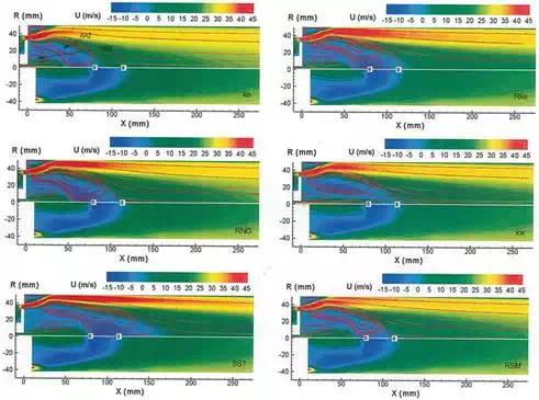
FIGURE 3.
Axial velocity contours and flow path lines.
Various degrees of agreement with the experimental data are illustrated among the six models for predicting the reattachment points or lengths of the ARZ and CRZ. As shown in the first plot for the standard k‐ε model, both ARZ and CRZ lengths are considerably under‐predicted. This type of shortcoming is also pointed out by other researchers for non‐reacting flow studies. The Rk‐ε model illustrates superior performance over the standard k‐ε model. It can properly predict the ARZ length and give a moderate result for the CRZ length. The RNG model underestimates the ARZ length slightly, but the CRZ length considerably. The results from the two k‐ω models are poorer than those from the Rk‐ε and RNG models. The k‐ω model underestimates the ARZ length, while overestimates the CRZ length. In terms of the SST model, it considerably over‐predicts the ARZ length though it gives a good result for the CRZ length. The RSM model, as shown in the last plot of Figure 3, illustrates the best performance, where both ARZ and CRZ lengths are satisfactorily provided.
A few parameters that may be valuable to combustion emission and stability studies can be obtained from the above RSM results. It is found that the gas mixture flow rate re‐circulated in the ARZ is equal to 5.5% of the total inlet airflow, and the ARZ length is 1.7 times longer than the diameter of the flame‐holder.
The axial velocity profiles along the combustor axis are illustrated in Figure 4 for the six turbulence models and compared with the experimental data. As shown in the figure, the peak value of measured negative axial velocity is −10 m/s, located at x ≈ 80 mm. The error bars representing 4% measurement accuracy are included in the figure. Considerable differences are found in the upper stream region from 10 to 80 mm for the k‐ε and k‐ω models, and in the downstream region from 80 to 360 mm for the k‐ε and SST models. The RSM, Rk‐ε and RNG models reasonably well predict the axial velocities along the central axis. Generally, the RSM gives the best results among the six turbulence models, which is consistent with the fact that only the RSM can adequately calculate both recirculation zones. For the five two‐equation models, the Rk‐ε illustrates better performance than the other four models.
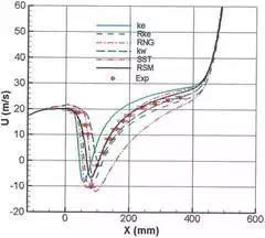
FIGURE 4.
Axial velocities along the combustor central axis.
The axial velocity profiles from x = 20 to 240 mm are displayed in Figure 5 at selected seven cross‐sections. Among these sections, three pass through the recirculation zones, one nearly cuts through the annular stagnation point and the remaining three are located further downstream. The features and magnitudes predicted from these models are generally close to the experimental measurements, but considerable differences are found at x = 40 – 200 mm sections for the k‐ε model, and x ≥ 160 mm downstream sections for the SST model. The best performance at the three upstream sections is given by the SST model because it adequately estimates the central recirculation zone, as shown in Figure 3. The results of the Rk‐ε and RNG models are close to those obtained from the RSM. The improvement of the RSM over the Rk‐ε model is observed in the regions of x = 120–200 mm and R = 30–40 mm.
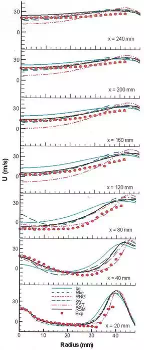
FIGURE 5.
Axial velocity profiles at cross‐sections, x = 20–240 mm.
The comparisons between the numerical and experimental results for the turbulence kinetic energy at four cross‐sections from x = 60 to 240 mm are presented in Figure 6, and the measurement accuracy of 8% is shown by error bars. Again, only the RSM provides encouraging predictions at all sections. In addition, the promising results of three normal turbulence stresses and one shear stress from the RSM model are also obtained. The numerical results agree reasonably well with the experimental data, particularly for the shear‐stress profiles.
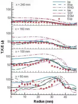
FIGURE 6.
Turbulence kinetic energy profiles at cross‐sections, x = 60–240 mm.
In Figure 6, the turbulence kinetic energy is considerably overestimated by the RNG model at all sections and the k‐ε model at the upstream sections. For the Rk‐ε and k‐ω models, except for the k‐ω model at section x = 100 mm, reasonable agreement with the experimental data is observed. The SST model fairly well predicts the turbulence kinetic energy in the central area, and however overestimates its value away from the combustor axis. These comply again with the above observation shown in Figure 3 that the SST model can properly calculate the CRZ, but fails to assess the ARZ. Note that since the x = 60 mm section crosses both recirculation zones where the two peak regions of turbulence kinetic energy are located, it represents a challenging task for numerical prediction. Unfortunately, none of these models can properly capture the central peak value.
In short, in terms of velocity flow‐field prediction, the RSM is superior over the five two‐equation models and in general, the Rk‐ε model illustrates better performance than the other four two‐equation models.
TEMPERATURE DISTRIBUTIONS
The upper halves of Figure 7 present the temperature contour results of the six turbulence models. The stoichiometric line of the mean mixture fraction is superimposed in each plot, and it starts from the edge of the disk flame‐holder, passes through the high‐temperature region and ends at the combustor axis. As illustrated in the figure, the flame is ignited at the downstream end of the flame‐holder edge and propagates downstream over the annular recirculation zone envelope. Along the envelope, the gaseous mixture of fuel and hot gas re‐circulated from downstream mixes with the fresh air from the inlet section and the combustion takes place. During the experimental testing, a carbon deposit was observed at the disk edge of the flame‐holder, which is consistent with the numerical prediction.
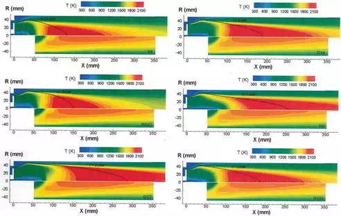
FIGURE 7.
Temperature contours and flow path lines.
The comparisons of the numerical results with the experimental data in the lower halves of Figure 7have shown that the size and location of the high‐temperature region are in good agreement with the experimental data for the RSM and Rk‐ε models, while the RSM performance is a little better than the Rk‐ε model. As shown in the figure, the standard k‐ε and RNG models underestimate high‐temperature region and the high‐temperature regions are shifted upstream. On the contrary, the k‐ω and SST models considerably overestimate high‐temperature region, and the high‐temperature regions are shifted downstream.
Figure 8 quantitatively compares the calculated temperature profiles along the combustor central axis with the experimental data, where the measurement error is about 5%. The calculated trends are close to the experimental values along the combustor central axis from 50 to 350 mm. However, in the central portion, the experimental profile is almost flat, while the predicted profiles display peak values. Overall, the better performance is given by the RSM and Rk‐ε models among the six models. The k‐ε and RNG models predict higher temperature than the experimental data in the upstream area and lower temperature in the downstream area. On the contrary, the k‐ω and SST models underestimate the temperature in the upstream and significantly overestimate it in the downstream.
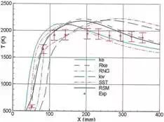
FIGURE 8.
Temperature profiles along the combustor central axis.
As indicated in Figures 7 and 8, the calculated temperatures are higher than the measured values in the centre region from x ≈ 140 to 250 mm, and the maximum deviation is about 150 K. Three reasons are anticipated. Firstly, as mentioned earlier, the temperature was measured by thermocouples. Due to the radiation and conduction heat losses from the thermocouple, the measurement error could be higher than 100 K at the locations where the flow velocity was low and the gas temperature was high. Secondly, the temperature probe could modify local flow structure, thus increases local turbulent mixing and causes an increase in local temperature. Thirdly, the turbulence kinetic energy (Figure 6) may not be properly calculated in the local region, and consequently the combustion and temperature calculation could be affected.
The temperature profiles at seven cross‐sections, x = 52–353 mm are presented in Figure 9 for the six models. For the RSM and Rk‐ε models, the predicted results agree reasonably well with the experimental data, besides the most upstream section and the small local area near the combustor wall. The RNG model illustrates the similar performance at sections from x = 82 to 293 mm. For the other three models, poor performance is found at upstream sections from x = 52 to 112 mm for the k‐ε model, x = 82, 232–353 mm sections for the k‐ω model, and most sections for the SST model.
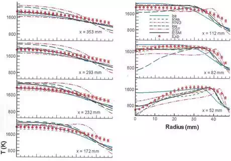
FIGURE 9.
Temperature profiles at cross‐sections, x = 52–353 mm.
Similar to the velocity predictions observed above, in general, the predicted temperature results from the RSM and Rk‐ε models fairly agree with the experimental data.
SPECIES DISTRIBUTIONS
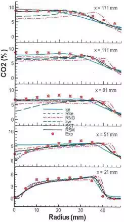
Figure 10 presents the CO2 mole fraction profiles at five cross‐sections, from x = 21 to 171 mm for six turbulence models, and compares them with the experimental data. These results are obtained with the flamelet combustion model (31 species) and the estimated error for species measurements is about 5%, as shown by error bars in the figure. The five cross‐sections are chosen to show the main trends of chemical reactions, that is two passing through the central recirculation zone, two across the annular recirculation zone and the last one after the recirculation region (see Figure 3).
FIGURE 10.
CO2 profiles at cross‐sections, x = 21–291 mm.
Carbon dioxide is one final major species of propane‐air combustion. The Rk‐ε and RSM predictions agree fairly well with the experimental data, except for the central region at x = 111 mm and the middle region at x = 81 mm, as illustrated in Figure 10. Poor prediction is found at x = 51 mm section for the k‐ε model, x = 81 and 171 mm sections for the k‐ω model and x = 171 mm section for the SST model.
Carbon monoxide, CO, is one major immediate species in hydrocarbon fuel combustion. The CO radial profiles are represented in Figure 11, where the numerical results are compared with the experimental data. Similar to the CO2 case, all models properly estimate the CO profile at the most upstream section, except for the SST model showing a small bump at R ≈ 38 mm. The RSM and Rk‐ε predictions agree fairly with the experimental data at x = 51 and 171 mm. It is found that the two models over‐predict the CO mole fraction in the central region, while under‐predict the CO2 at the two other sections, x = 81 and 111 mm. However, the sum of CO2 and CO of the predicted results is close to the sum of the experimental data for CO2 and CO. This indicates that the calculated oxidization of CO at these two sections is lag behind. Poor prediction is found again for the k‐ε model at section x = 51 mm, k‐ω model at section x = 171 mm and SST model at sections x = 111 and 171 mm.
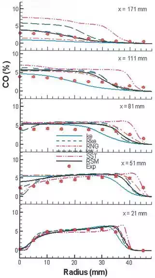
FIGURE 11.
CO profiles at cross‐sections, x = 21–291 mm.
In brief, the Rk‐ε and RSM results are consistent with the experimental data except for some local regions, and better than the other models. The species predictions are encouraging in general.
The above qualitative and quantitative comparisons of velocity, temperature and species distributions inside the combustor between the numerical results and experimental database clearly indicate that the RSM model, a second‐moment closure, is better than the eddy‐viscosity models. This agrees with the findings from other authors, such as for a non‐reacting flow and for a reacting flow. Furthermore, the Rk‐ε model illustrates better performance than other four two‐equation models. Instead of the RSM, utilization of the Rk‐ε model for practical gas turbine combustor simulations can avoid some numerical problems, such as stability and time‐consuming issues.
For the SST model, it can provide good solutions in many non‐reacting flows, such as the NACA 4412 air foil, backward‐facing step and adverse pressure gradient flows. However, the model considerably overestimates the high‐temperature region and annular recirculation zone in the combustion chamber and this type of result is also found in the simulations of a real‐world gas turbine combustor Two reasons are anticipated. Firstly, the testing cases used for model validation are isothermal or almost isothermal flows, and the considerable thermal expansion and chemical reaction may not be adequately accounted for in the model This may justify that the features in the central recirculation zone can be appropriately estimated by the SST model, as seen from Figures 3, 5and 6, because the temperature is low in the central recirculation zone, as seen from Figure 7. Secondly, multiple large vortices or recirculation regions play an important role in fuel‐air mixing and combustion management in the combustion chamber, and this type of flow is more complex than single vortex flows, such as the backward‐facing step flow. For example, in the present case, the whole central recirculation zone is buried inside the annular recirculation zone.
Application of Reynolds analogy
Most of these results are obtained with the RSM turbulence model and PDF combustion model. By comparing the numerical results with the experimental database, the Reynolds analogy approach can be assessed and the optimized turbulence Prandtl/Schmidt number for the combustor flow‐fields can be identified.
VELOCITY DISTRIBUTIONS
The predicted axial velocity contours are illustrated in Figure 12 for Lt = Prt = Sct = 0.85, 0.50 and 0.25, respectively, and compared with the experimental data. The flow patterns in the combustion chamber are well captured in all three plots and two reattachment points or lengths of the two recirculation zones are properly predicted.
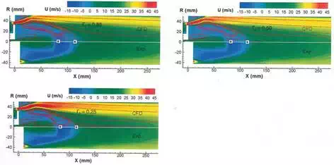
Axial velocity contours and flow path lines, Γt = 0.85, 0.50 and 0.25.
As mentioned earlier, turbulence scalar transfers are calculated based on the modelled turbulent momentum transfer, and however the former may also affect the latter since they are coupled. As shown in Figure 12, the effect of Γt on velocity field for Γt = 0.85–0.25 is minor. For Γt = 0.25, the length and volume of the annular recirculation zone are slightly reduced in comparison with those from Γt = 0.50 and 0.85.
The similar trends for the axial velocity profiles along the combustor central axis, and the axial velocity, turbulence kinetic energy and shear‐stress profiles at a number of cross‐sections are also observed. These results indicate that the effect of Гt variation on the predicted velocity field is minor, and the predicted velocity fields agree fairly well with the experimental data for Гt > 0.35.
TEMPERATURE DISTRIBUTIONS
The temperature contours for Гt = 0.85, 0.50 and 0.25 are presented and compared with the experimental database in Figure 13. Strong turbulent mixing makes the temperature in the recirculation region relatively uniform. Along the envelope of the annular recirculation zone, combustion occurs intensively. In comparison with the experimental data, for the large Гt number of 0.85, the high‐temperature region is enlarged and shifted downstream, while for the small Гt number of 0.25, the high‐temperature region is considerably reduced and shifted upstream. The best results are observed for Гt = 0.50. Generally, as Гt decreases, the turbulence transfers of fuel into the airflow and then the chemical reaction are enhanced. As a result, the high temperature region is smaller and shifts upstream. Figure 13shows that the predicted maximum temperature in the high temperature region is higher than the measured values, which has been explained earlier.
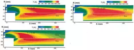
FIGURE 13.
Temperature contours, Гt = 0.85, 0.50, 0.25.
Figure 14 illustrates the effect of Гt on the predicted flame length. In the upper plot, the stoichiometric line of the mean mixture fraction (f˜=0.0603f˜=0.0603) is used to signify the flame length, and in the lower plot, the OH mole fraction contour lines are employed. The effect of Гt on the flame volume or length is clearly observed. Both the flame volume and length are substantially decreased as Гt decreases from 0.85 to 0.25, and the flame length reduces more than three times from 365 to 110 mm.
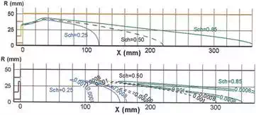
FIGURE 14.
Variation of predicted flame length with Гt.
The predicted temperature profiles along the combustor central axis are compared with the experimental data in Figure 15. The limited effect of Гt is shown in the upstream region (x < ∼80 mm); the predicted values for Гt = 0.50 and 0.85 agree well with the measured data. Conversely, the strong effect of Гt is observed in the downstream region. This is because the fuel distribution or chemical reaction in the upstream region is mainly controlled by the size and location of the annular recirculation zone, which is created by complex flow interactions among the central fuel jet, annular airflow and two recirculation zones. In other words, the flow field is dominated by convection. However, the turbulent diffusion or transfer in the downstream region plays a major role in the fuel spreading away from the axis of symmetry, as shown in Figure 12 where the flow path lines are almost parallel to each other. As shown in Figure 15, Гt = 0.50 gives the best results although the predicted profile shows a peak in the middle portion, while the measurements tend to be flat.
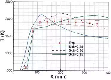
FIGURE 15.
oTemperature profiles along the combustor central axis.
Figure 16 presents the temperature profiles for Гt = 0.85, 0.50 and 0.25 at five cross‐sections from x = 52 to 233 mm. The temperature profiles become flatter or the fuel spreading becomes faster as Гtdecreases at all sections. Generally, the predicted results for Гt = 0.50 are close to the measured data, except for the local regions around the combustor wall. In these near‐wall regions, the temperature is underestimated and it may indicate the under‐prediction of fuel spreading in these regions. Poor prediction is found for Гt = 0.25 at sections x = 82 and 233 mm, and Гt = 0.85 at section x = 52 mm. The effect of Гt is strong at all five sectins.
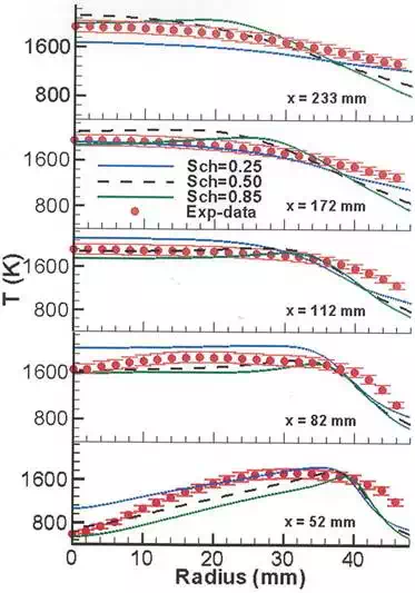
FIGURE 16.
Temperature profiles at sections x = 52–233 mm.
WALL TEMPERATURE DISTRIBUTION
Variation of combustor wall temperature with Гt is shown in Figure 17, and the numerical results are evaluated against the experimental data. Unsurprisingly, the predicted wall temperature increases as Гtdecreases. The best agreement with the experimental data is obtained with Гt = 0.35 although the wall temperature is a little overestimated in the upstream region and underestimated in the downstream region. Note that this Гt number is different from the preferred value of 0.50 for the temperature prediction inside the combustor as discussed earlier. It may indicate that instead of a constant number, varying Гt should be considered in turbulent reacting flow simulations.
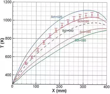
FIGURE 17.
Temperature profiles along the combustor wall.
In order to thoroughly assess the Reynolds analogy issue, numerical simulations were also carried out with the eddy‐dissipation (EDS) and laminar flamelet combustion models. A large amount of numerical results and figures were generated, with a Гt increment of 0.05 or even 0.01. The trends and magnitudes of velocity, turbulence kinetic energy, Reynolds stresses and temperature distributions are similar to those obtained from the PDF combustion model. Although the results are not presented in this chapter, the optimized Гt numbers are given in Table 1 for the purpose of comparison.
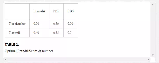
As shown in the above results, the optimal Гt number for the temperature prediction inside the combustor is 0.50 for all three combustion models. This number is different from 0.20 and 0.25 for gas turbine combustor studies, and 0.20 for a cross‐jet flow simulation [25]. However, it is the same as recommended by Syed and Sturgess for recirculation zone simulations.
Two important facts are revealed from the above all examples. Firstly, the Гt number optimized is smaller than the conventionally accepted value of 0.6–0.85. Secondly, most likely the combustor configuration and possibly the operating conditions affect the optimal value of Гt. Therefore, a priori optimization of Гt is preferred in order to confidently predict temperature and species distributions inside combustors.
These observations may be attributed to the following reasons. Firstly, theoretically, Eqs. (11)–(13) are only valid for boundary layer flows, where the streamwise pressure gradient, viscous and source terms can be neglected. Certainly, its application to complex turbulent reacting flows is questionable. Secondly, the experimental numbers of Гt (∼0.7) are measured from fully developed boundary or pipe flows [12, 13, 63], which are quite different from practical three‐dimensional turbulent reacting flows. In terms of the relative strength between the turbulence momentum and scalar transfers for the numerical methods and models used today, a low value of Гt is true, and it may change with flow configurations.
Thirdly, the gradient‐type diffusion assumption used in Eqs. (11)–(13) has been questioned by a large number of researchers, in particular for turbulent energy and heat transfer. As pointed out in Ref. [12], to adequately model turbulence scalar transfers, not only the gradient‐based diffusion from small‐scale turbulence, but also the convection effect from large‐scale turbulent motion should be taken into consideration. This may imply that the gradient‐based diffusion method is appropriate for turbulent boundary flows, but it may not be proper for complex flows, such as practical combustion systems.
As a summary, the Reynolds analogy approach has been applied to general three‐dimensional flow‐field simulations from the 1970s. In order to accurately predict the turbulence scalar transfers without a prior optimization, the improvement of the current approach is necessary, and new ideas should be considered.
Conclusions
Turbulence modelling is one of major issues, which affects the precision of current numerical simulations in engineering applications, particularly for reacting flows. To systematically study and validate various physical models, a series of experimental measurements have been carried out at the National Research Council of Canada on a model combustor, and a comprehensive database has been obtained. The combustor simulations with the interior and exterior conjugate heat transfers have been carried out with six turbulence models, i.e. the standard k‐ε, re‐normalization group k‐ε, realizable k‐ε, standard k‐ω, shear‐stress transport (SST) and Reynolds stress models. The laminar flamelet, PDF and EDS combustion models and the discrete ordinate radiation model as well are also used.
All six turbulence models can capture the flow features or patterns; however, for the quantitative predictions of velocity, temperature and species fields, different levels of performance are revealed. The RSM model gives the best performance, and it is the only one that can accurately predict the lengths of both recirculation zones and offer reasonable prediction on the turbulence kinetic energy distribution in the combustor. In addition, the performance of the Rk‐ε model is better than other four two‐equation models, and it can give similar results as those from the RSM under the present configuration and operating conditions.
The effect of the turbulent Prandtl/Schmidt number on the flow field of the model combustor has also been numerically studied. In this chapter, some of the results obtained with turbulent Prandtl/Schmidt number varying from 0.85 to 0.25 have been presented and discussed. It has a strong effect on the temperature fields, particularly downstream in the combustor. This is also true for the temperature profile along the combustor wall. On the contrary, its effect on the velocity field is limited.
For all three combustion models, the optimal Гt is 0.5 for temperature prediction in the combustor, while for predicting temperature at the combustor wall the optimal value alters from 0.35 to 0.50. With Гt = 0.50, except for some local regions, the velocity, temperature and major species fields in the combustor are fairly well simulated.
As a final point, considering the foundation and shortcoming of the Reynolds analogy, to accurately predict temperature and species distributions in turbulent reacting flow fields without an optimization of turbulent Prt and Sct numbers, the Reynolds analogy approach should be enhanced and new ideas should be considered.
