Interface Instability and Turbulent Mixing
Abstract
Richtmyer‐Meshkov instability and turbulent mixing are fundamental problems of multi‐materials interface dynamics, which mainly focuses on the growth of perturbation on the interface and mixing of different materials. It is very important in many applications such as inertial confinement fusion, high‐speed combustion, supernova, etc. In this chapter, we will gain advances in understanding this problem by numerical investigations, including the numerical method and program we used, the verification and validation of numerical method and program, the growth laws and mechanics of turbulent mixing, the effects of initial conditions, the dynamic behavior, and some new phenomenon for Richtmyer‐Meshkov instability and turbulent mixing.
Introduction
When a shock wave accelerates a perturbed interface separating two different fluids, the Richtmyer‐Meshkov (RM) instability will occur. This phenomenon was theoretically analyzed by Richtmyer [1] for the first time in 1960, which was confirmed in experiment by Meshkov [2] in 1969. The main mechanism of the Richtmyer‐Meshkov instability (RMI) is the baroclinic vorticity deposition at the interface due to the misalignment of the pressure gradient across the shock and the local density gradient at the interface (∇ρ × ∇p ≠ 0). At the beginning, the perturbations grow linearly. When entering the nonlinear stage, the perturbations develop into complex structures formed by bubbles (the portion of the light fluid penetrating into the heavy fluid) and spikes shaped with “mushrooms” (the portion of the heavy fluid penetrating into the light fluid), see Figure 1. Afterward, the mushroom structures are eroded and broke up which results in the turbulent mixing eventually. When the incident shock wave impacts the initial perturbed interface, it bifurcates into a transmitted shock wave and a reflected wave. Depending on the material properties of the fluid on both sides of the interface, the reflected wave can be either a shock or a rarefaction wave. The criterion is that when the incident shock wave interacts with the interface from light fluid to heavy fluid, the reflected wave is a shock wave; otherwise, it is a rarefaction wave. If the transmitted shock wave meets a rigid wall and is reflected back to collide with the interface once again, this process is called reshock which can advance the transition to turbulent mixing.
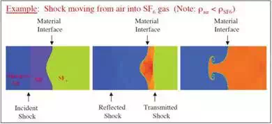
FIGURE 1.
Development of the Richtmyer‐Meshkov perturbed interface between air and SF6 gases [3].
The Richtmyer‐Meshkov instability and induced turbulent mixing are very important in a variety of man‐made applications and natural phenomena such as inertial confinement fusion (ICF) [4], deflagration‐to‐detonation transition (DDT) [5], high‐speed combustion [6], and astrophysics (i.e., supernova explosions) [7]. For ICF, the ablative shell that encapsulates the deuterium‐tritium fuel becomes RM unstable as it is accelerated inward by the ablation of its outer surface by laser or secondary X‐ray radiation. The degree of compression achievable in laser fusion experiments is ultimately limited by Richtmyer‐Meshkov and Rayleigh‐Taylor instabilities. Thus, these instabilities represent the most significant barriers to attaining positive‐net‐yield fusion reactions in laser fusion facilities. For the supersonic combustion, the Richtmyer‐Meshkov instability caused by the interaction of a shock wave with a flame front can greatly promote the mixing of fuel and oxidant and enhance the burning rate. For the supernova explosions, the Richtmyer‐Meshkov instability was believed to occur when the outward propagating shock wave generated by the collapsing core of a dying star passes over the helium‐hydrogen interface. Observations of the optical output of the supernova 1987A suggest that the outer regions of the supernova were much more uniformly mixed than expected, and indicating significant Richtmyer‐Meshkov mixing had occurred [8]. The Richtmyer‐Meshkov instability and turbulent mixing are so important and have gained significant attention. However, the turbulent mixing is a complicated three‐dimensional unstable flow, which spans a wide range of time‐space scales.
Numerical method and program
By applying the piecewise parabolic method (PPM), volume of fluid (VOF), parallel technique, and so on, we have developed a series of Euler compressible multi‐fluid dynamic programs with three orders precision, such as MFPPP [9], MVPPM [10], and multi‐viscous‐flow and turbulence (MVFT) [11, 12]. MFPPM program is not considering the fluid viscosity, which only solves the Euler equations. MVPPM program is considering the molecular viscosity but it is not changed with temperature. Multi‐viscous‐flow and turbulence (MVFT) is a large‐eddy simulation (LES) program that has four choices of subgrid‐scale (SGS) stress models including the Smagorinsky model [13], Vreman model (VM) [14], dynamic Smagorinsky model (DSM) [15], and stretched‐vortex model (SVM) [16].
GOVERNING EQUATIONS
The governing equations of large‐eddy simulation are the Favre‐filtered compressible multi‐viscous‐flow Navier‐Stokes (NS) equations and are written as in tensor form:
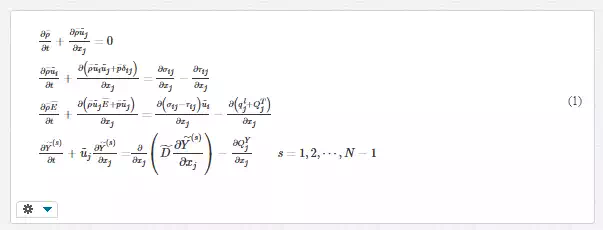
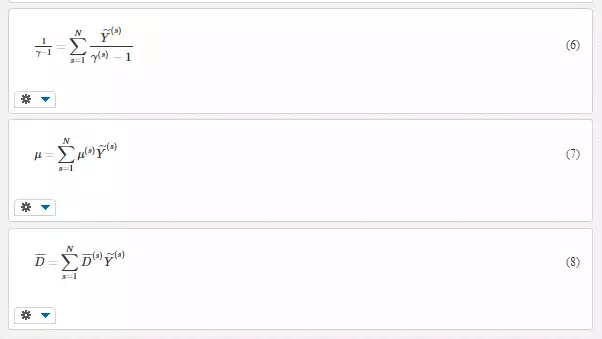
here i and j represent the directions of x, y, and z, and the same subscripts denote the tensor summation; ρ¯ρ¯, u˜k(k=i,j)u˜k(k=i,j), p¯p¯, and E¯¯¯E¯ are the resolved‐scale density, velocity, pressure, and total energy per unit mass; N is the number of species; Y˜(s)Y˜(s) is the volume fraction of the sth fluid and satisfies ∑N1Y˜(s)=1∑1NY˜(s)=1; D˜D˜ is the diffusion coefficient set to D˜=ν/ScD˜=ν/Sc, where ν is the kinematic viscosity of the fluid, Sc is the Schmidt number. σij is the deviatoric Newtonian stress tensor, i.e.
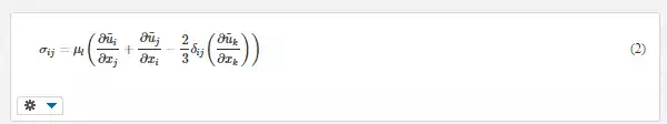
where μl is the dynamic viscosity. qlj=−λl∂T˜/∂xjqjl=−λl∂T˜/∂xj is the resolved heat transport flux per unit time and space, λl = μlcp/Prl is the resolved heat conduction coefficient, cp is the constant pressure specific heat, Prl is the Prandtl number, and T˜T˜ is the fluid temperature. The equation of state (EOS) has choices of the ideal gas state form, stiffen gas state form, reduction form of Gruneisen EOS for condensed matter.
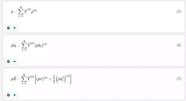
For a multi‐material mixture case, the average quantities and physical properties of a mixed phase are supposed as a volume‐weighted sum over the set of components (ρ¯)(s)(ρ¯)(s), (ρ¯u˜i)(s)(ρ¯u˜i)(s), and (ρ¯E˜)(s)(ρ¯E˜)(s) used at the initial time, and so on for each, respectively,
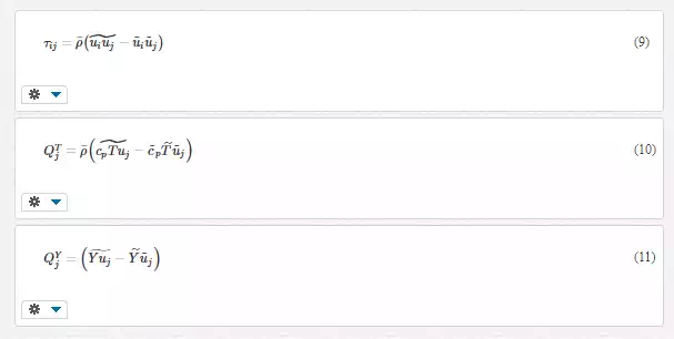
For large‐eddy simulation, in the filtering operation, the unresolved‐scale motions identified as the “subgrid‐scale” are filtered, but the effects of subgrid‐scale motions on the resolved‐scale motions are retained in the governing equations in the form of SGS turbulence transport fluxes, which must be modeled to complete the closure of LES equations. The SGS stress tensor, the heat, and scalar transport flux are defined as
SUBGRID‐SCALE STRESS MODELS FOR LES
SMAGORINSKY MODEL
The SGS turbulence behavior is assumed to be analogous to the molecular dissipative mechanism, so that the molecular viscosity and diffusion models can be used to simulate the SGS fluxes, and the SGS stress tensor, the heat, and the scalar transport flux are calculated as follows [13]
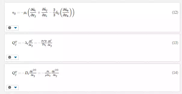
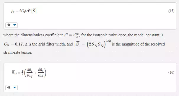
where the SGS turbulent viscosity μt is calculated by the Smagorinsky eddy viscosity model,
VREMAN MODEL
The Vreman SGS model is also an eddy viscosity model and is as follows [14]:
DYNAMIC SMAGORINSKY MODEL
In general, the turbulent kinetic energy is transferred from large scales to small scales in turbulent flows, which is called forward scatter of energy, and then it is dissipated by the viscous action. However, the reversed energy flow from small scales to large scales (the process called backscatter) may also occur. Although the backscatter is just a small range of local phenomenon, it has been shown to be of importance, especially in the transition regime. The physical mechanism of most of the widely used SGS models is the forward scatter of energy; in other words, the SGS models are absolutely dissipative, such as the eddy viscosity models (Smagorinsky and Vreman SGS models). In order to account for the backscatter of energy,
several modifications to the eddy viscosity models have been proposed. An improvement is to calculate the eddy viscosity coefficient dynamically which is a function of space and time and can be negative in some regions [15].
The dynamic Smagorinsky model for compressible turbulence is as
follows, the model coefficient is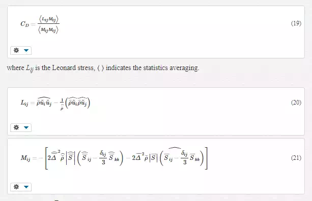
the overbars of “¯” and “^” denote the grid filter and test filter, respectively.
STRETCHED‐VORTEX MODEL
The stretched‐vortex model is based on an explicit structural modeling of small‐scale dynamics. It can simulate the multiscale compressible turbulence and allows the anisotropy of the flow to be extended to the dissipation scale. In the stretched‐vortex model, the flow within a computational grid cell is assumed to result from an ensemble of straight, nearly axisymmetric vortices aligned with the local resolved scale strain or vorticity. The resulting SGS flux terms are [16]
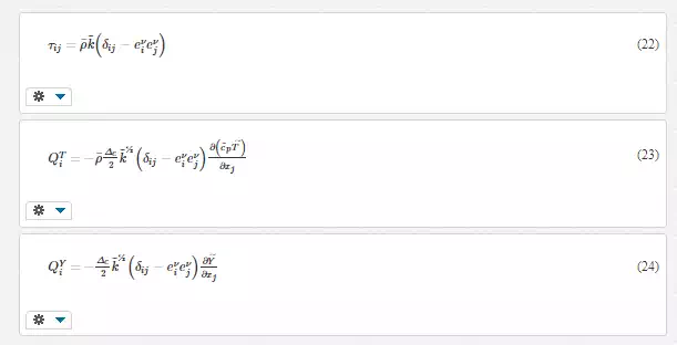
where k˜=∫∞kcE(k)dkk˜=∫kc∞E(k)dk is the subgrid turbulent kinetic energy, eν is the unit vector aligned with the subgrid vortex axis, kc=π/Δckc=π/Δc is the cutoff wave number, E(k)=K0ε2/3k−5/3exp[−2k2ν/(3|a˜|)]E(k)=K0ε2/3k−5/3exp[−2k2ν/(3|a˜|)] represents the energy spectrum of subgrid vortices, and K0is the Kolmogorov prefactor, ε is the local cell‐averaged dissipation, a˜=S˜ijeνieνja˜=S˜ijeiνejν is the axial strain along the subgrid vortex axis, S˜ijS˜ij denotes the resolved rate‐of‐strain tensor.
NUMERICAL ALGORITHM
For the convenience, in the following sections, the overbar and overtilde of variables are omitted. Operator splitting technique is used to solve the physical problems, described by Eq. (1), into three sub‐processes, i.e., the computation of inviscid flux, viscous flux, and heat flux. Eq. (1) can be split into two equations as follows:
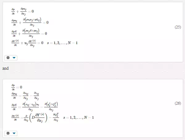
For the inviscid flux, the three‐dimensional problem can be simplified into one‐dimensional (1D) problem in three directions of x, y, and z by the dimension splitting technique,
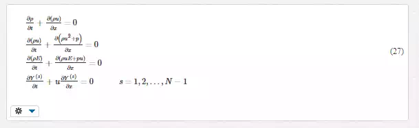
And then the one‐dimensional Eq. (27) in each direction is resolved by the two‐step Lagrange‐Remapping algorithm. Also, one time step is divided into four substeps: (i) the piecewise parabolic interpolating of physical quantities, (ii) solving the Riemann problems approximately, (iii) marching of the Lagrange equations, and (iv) remapping the physical quantities back to the stationary Euler meshes. The orders of accuracy of the spatial and temporal schemes are the third and second, respectively, for smooth flows.
LAGRANGE STEP OF FINITE VOLUME METHOD
The Lagrange equations in 1D for multi‐fluid can be written as
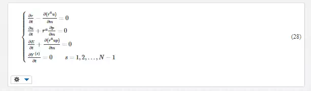
where τ is the specific volume, α is 0, 1, and 2 corresponding to the plane, axial symmetry, and spherical symmetry problems, r is the Lagrange spatial coordinates, m is the Lagrange mass coordinates m=∫rr0ρrαdrm=∫r0rρrαdr, u=∂r∂tu=∂r∂t, mj−1/2 and mj+1/2 are the mass coordinates of both sides of the jth grid, Δm = mj+1/2 − mj−1/2. The mass average of physical quantities (τ,u,E,Y(s))nj(τ,u,E,Y(s))jn for the jth grid can be defined as
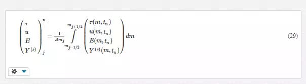
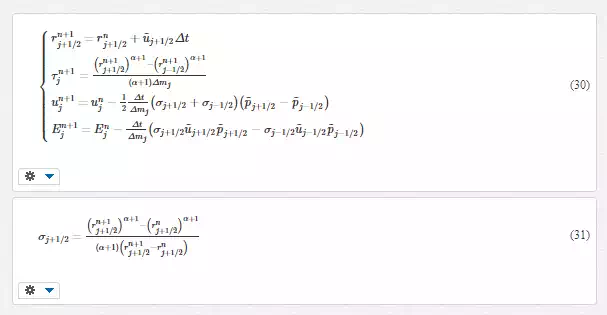
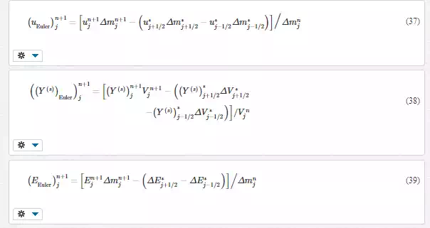
Because of the calculations are referred to as scalars, here the averaged physical quantities in a cell are written as a uniformity QnjQjn at time t. The piecewise parabolic function Qnj(m)Qjn(m) in cells are constructed to compute the time average of physical quantity Q on both sides of the grid edge mj+1/2,Q˜j+1/2,LQ˜j+1/2,L and Q˜j+1/2,RQ˜j+1/2,R. Then the Riemann problem at the grid edge mj+1/2 is solved by using double shock wave approximation. After Lagrange marching step, we can obtain distribution of the physical quantities {τn+1j},{un+1j},{En+1j},{τjn+1},{ujn+1},{Ejn+1}, and the position of new grids {rn+1j±1/2}{rj±1/2n+1} at time tn+1, the pressure {pn+1j}{pjn+1} can be computed by equation of state, the {(Y(s))n+1j}{(Y(s))jn+1} will not change. The marching formula is as follows
REMAP STEP
In Lagrange step, the computational cells distort to follow the material motion, and in Remap step, the averaged physical quantities at the distorted Lagrange cells are remapped back to the stationary Euler meshes. The piecewise parabolic interpolation and integral methods in this step are the same as the ones in Lagrange step.
After Remap step, we define the physical quantities in Euler mesh as (ρEuler)n+1j,(ρEuler)jn+1, (uEuler)n+1j,(uEuler)jn+1, (EEuler)n+1j,((Y(s))Euler)n+1j(EEuler)jn+1,((Y(s))Euler)jn+1, the volume of fluid through the grid boundary j+1/2j+1/2 as ΔV∗j+1/2ΔVj+1/2*, and the average of physical quantities as (ρ∗,u∗,p∗,(Y(s))∗)j+1/2(ρ*,u*,p*,(Y(s))*)j+1/2. The density after Lagrange step is ρn+1j=1/τn+1jρjn+1=1/τjn+1. In Remap step
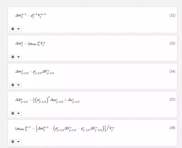
where Δe∗j+1/2Δej+1/2* is the advection of specific energy through the grid boundary j+1/2j+1/2.
VISCOUS FLUX, HEAT FLUX, AND SCALAR FLUX
The viscous flux, heat flux, and scalar flux of Eq. (26) are calculated based on the computed inviscid flux by using second‐order spatial center difference and two‐step Runge‐Kutta time marching. The first equation of Eq. (26) can be neglected, and which is written in conserved form
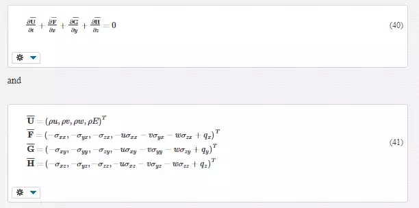
In the Cartesian coordinate system, the spatial derivative terms of Eq. (40) can be dispersed as follows
Verification and validation
In this section, the validity and reliability of our compressible multi‐fluid dynamic programs are to be verified and validated by comparisons with analytical solutions and hydrodynamic interface instability experiments in a shock tube.
RIEMANN PROBLEM OF CONDENSED MATTER
A copper pellet collides with a copper target with three velocities of 2, 4, and 8 km/s. Using the reduction form of Gruneisen EOS for copper in simulations, the one‐dimensional numerical results of postshock density (a), pressure (b), and velocity (c) compare with theoretical solutions, as shown in Figure 2, the solid lines corresponding to numerical results and the dot lines corresponding to the theoretical solutions.
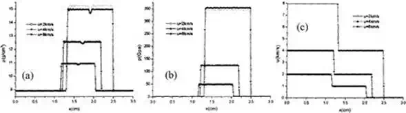
FIGURE 2.
Comparison of postshock density (a), pressure (b), and velocity (c) in copper at t = 1.0 μs when a copper pellet collides with a copper target at three different velocities.
RIEMANN PROBLEM OF ONE‐DIMENSIONAL GAS/LIQUID
At initial time, the region [0, 1.0 cm] is filled with gas with high pressure 1.0 × 10⁸ Pa and density 1.29 g/cm3. The region [1.0 cm, 5.0 cm] is filled with water with pressure 1.0 × 10⁵ Pa and density 1.0 g/cm3. The gas and water are all described by Stiffen gas EOS. The left and right boundaries are flow. Figure 3 shows the distributions of the density (a), pressure (b), and velocity (c) at 20 μs. There are a forward shock wave and a backward rarefaction wave after interaction. The pressure and velocity around the interface are well continuous and have no nonphysical oscillation.
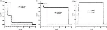
FIGURE 3.
Distributions of the density (a), pressure (b), and velocity (c) at 20 μs for one‐dimensional Riemann problem of gas/liquid interface.
SINGLE‐MODE RICHTMYER‐MESHKOV INSTABILITY
The two‐ and three‐dimensional single‐mode Richtmyer‐Meshkov instabilities are numerical simulated by MVPPM program, which also compare with the theoretical model [18]. The initial small perturbation is a sinusoidal one with wavelength 60 mm (global wavelength for a three‐dimensional case) and amplitude 1.0 mm. The incident air shock wave with Mach number 1.2 impacts the air/SF6single‐mode interface. Figure 4 shows the comparisons of amplitude of single‐mode perturbed interface with the linear impulsive and nonlinear models, the left one corresponding to the two‐dimensional (2D) results, and the right one corresponding to the three‐dimensional results.
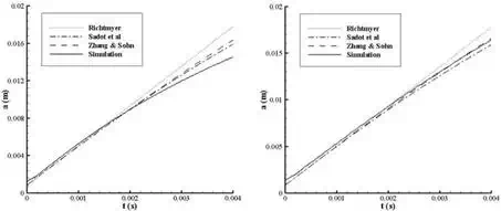
FIGURE 4.
Comparisons of amplitude of single‐mode perturbed interface with the linear impulsive model and nonlinear models, left: two‐dimension and right: three‐dimension.
SIMULATIONS OF SHOCK TUBE EXPERIMENTS
The compressible multi‐fluid dynamic programs are used to simulated several shock tube experiments of interface instability for validation. These experiments include planar interface and gas cylinder shock tube experiment and planar and cylindrical jelly experiments.
Figure 5 shows the comparison of 2D calculated width of turbulent mixing zone (TMZ) [19] of Leinov’s shock tube experiment with reshock with experiment [20] in which the Mach number of incident air shock wave is 1.2, which impacts the air/SF6 interface, the grid size is 50 μm. Figure 6shows the 3D calculated TMZ width [21] of Poggi’s multi‐mode shock tube experiment [22] with reshock in which the Mach number of incident SF6 shock wave is 1.453, which impacts the SF6/air interface. Figures 7 [10] and 8 [23] show the calculated and experimental interface images of AWE’s SF6 half‐height and double‐bump shock tube experiment [24, 25], the Mach number of incident air shock wave is 1.26, respectively. Figure 9 [26] shows the SF6 gas cylinder evolution at different times under the initial air shock wave with the Mach number 1.2, Figure 10 shows the width and height of gas cylinder at different times for experiment and numerical simulations.
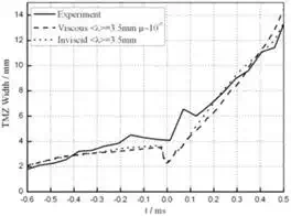
FIGURE 5.
TMZ width versus time (t = 0 denotes the reshock arrival to the interface).
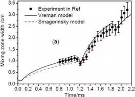
FIGURE 6.
Time history of TMZ width.
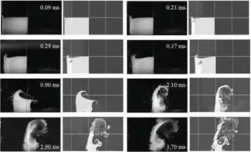
FIGURE 7.
Two dimension calculated from MVFT and experimental half‐height interface at different times
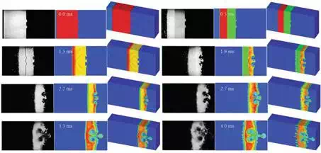
FIGURE 8.
Three dimension calculated from MVFT and experimental double‐bump interface at different times, left column corresponding to experimental images, right column corresponding to 3D calculated images, and middle column corresponding to span‐wise average images of 3D calculated results.
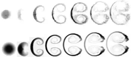
FIGURE 9.
Evolutions of SF6 gas cylinder, upper row corresponding to experiment, lower row corresponding to numerical simulation by MVFT program, the time sequences are 0, 50, 190, 330, 470, 610, and 750 μs severally.
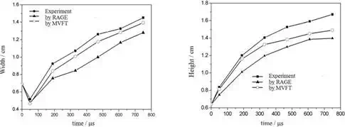
FIGURE 10.
Width and height of gas cylinder at different times for experimental and numerical simulations.
For the problems of interface instability with a high density ratio, our hydrodynamic programs are also applicable. For the LLNL’s jelly ring experiments [27], the jelly ring only has a sinusoidal periodic initial perturbation at the outer interface and is driven by expansion of the explosion products of a gaseous mixture of C2H2 and O2. The jelly is mainly made of water. The thickness of ring is 15 mm, the mode number of perturbation is 6 and 36, respectively, and the initial amplitude is 1.0 mm. Figure 11shows the evolutions of the jelly ring at different times from simulated from LLNL’ CALE program (a) and our MVPPM program (b), and the experimental image (c) at 600 μs [28]. Figure 12 shows the time histories of radius (a) and the amplitude (b) of the outer and inner interfaces of the jelly ring simulated from CALE and MVPPM programs [28]. Figure 13 shows the images of jelly ring at 600 μs for mode number 36 from experiment (a), CALE (b), and MVPPM (c) programs [28].
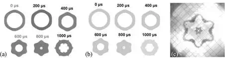
FIGURE 11.
Evolutions of jelly ring at different simulated from CALE (a: left group) and MVPPM (b: middle group) programs, and the experimental image at 600 μs (c).
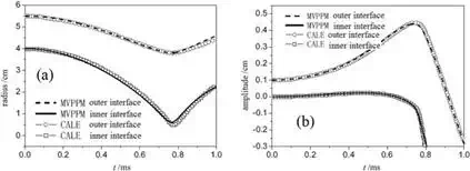
FIGURE 12.
Time histories of radius (a) and the amplitude (b) of the outer and inner interfaces of jelly ring simulated from CALE and MVPPM programs.
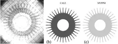
FIGURE 13.
Images of jelly ring at 600 μs for mode number 36 from experiment (a), CALE program (b), and MVPPM program (c).
From the above comparisons between our numerical simulations and theoretical model, experiments for the problems of hydrodynamic interface instability from the density ratio low to the high density ratio, the numerical results agree well with theory and experiments, so the validity and reliability of our compressible multi‐fluid dynamic programs have been verified and validated.
Interface instability and turbulent mixing
As we know, the physical mechanism for the occurrence of Richtmyer‐Meshkov instability is the baroclinic vorticity deposition at the interface resulting from the misalignment of the pressure gradient across the shock front and the local density gradient across the interface. The evolution equation of vorticity is as follows:
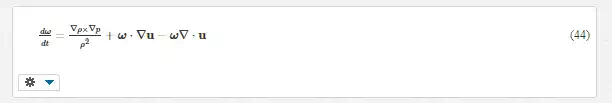
where ω = ∇ × u is the vorticity and viscous terms are neglected. The first term on the right side of Eq. (44) is the baroclinic vorticity production term. The second term on the right side of Eq. (44) is the vortex‐stretching term, which is zero in the two‐dimensional case, as the vorticity and velocity fields are orthogonal. This term enhances dissipation, resulting in more diffuse and smaller scale structures in the turbulent mixing zone. The third term on the right side is the compression term and does not contribute to the vorticity evolution significantly. The baroclinic vorticity production is much larger when the shock wave impacts the interface and pass through it and constitutes the principal mechanism of the Richtmyer‐Meshkov instability.
In this section, we will introduce the growth laws of the Richtmyer‐Meshkov instability and the induced turbulent mixing and its dynamic behavior by numerical simulations.
GROWTH LAWS OF RICHTMYER‐MESHKOV INSTABILITY AND TURBULENT MIXING
Figure 14 shows the amplitude (a) and growth rate (b) of two‐dimensional single‐mode Richtmyer‐Meshkov instability without reshock for initial perturbation amplitude 1 and 12 mm and wavelength 60 mm. After initial shock, the perturbation enters the nonlinear stage quickly. The growth rate increases fast and reaches the highest peak, then will reduce owing to the reduction of the effect of compressibility and the dominant role of flow nonlinearity. At the late times, the amplitude is increasing linearly, and the growth rate remains a constant. For the larger initial amplitude, the perturbation enters the later linear growth stage earlier.
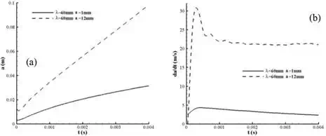
FIGURE 14.
Amplitude (a) and growth rate (b) of two‐dimensional single‐mode Richtmyer‐Meshkov instability without reshock.
For the multi‐mode Richtmyer‐Meshkov instability and the induced turbulent mixing with reshock, the initial air shock wave with Mach number 1.2 impacts the air/SF6 interface. The multi‐mode initial perturbation is composed of eight dominant mode wavelengths of 0.8, 1.0, 1.25, 1.6, 2.0, 2.5, 3.2, and 4.0 mm superimposed with a very small random disturbance. The shock tube experiment can be referred to Ref. [29]. Figure 15 shows the schematic of shock tube and computational model. The transmitted wave rebounds between the interface and the end‐wall of shock tube and produces multiple shock‐interface interactions. At about 1.7 ms, the transmitted shock wave reflected back off the end‐wall impacts the interface. Figure 16 shows the time history of TMZ width, the black line denotes the numerically calculated width and the red line is obtained from fitting of the numerical results. As can be seen, after the initial shock, the TMZ width starts to grow as a power law ;tθ with the value θ to be determined as 0.352. After the reshock, more energy is deposited onto the interface to promote the development of TMZ, and the TMZ width evolves in time as a negative exponential law ;−e−t/t∗−e−t/t*where the value of t* is 0.519. Then after the following interaction of the reflected rarefaction wave with the interface, the TMZ also evolves as a negative exponential law but with a different factor t* = 0.875. Under the subsequent impingements with lower and lower intensity, the TMZ width, after a slight reduction caused by the reflected compression wave, evolves in an approximate linear fashion with a velocity of 2.05 m/s. Figure 17 shows the instantaneous images of the TMZ visualized by the volume fraction isosurface YSF6 = 0.1, 0.3, 0.5, 0.7, and 0.9 from blue to orange at different times, the TMZ exhibits a very complex spatial structure.
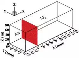
FIGURE 15.
Schematic of shock tube and computational model
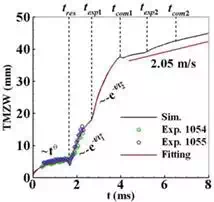
FIGURE 16.
Time history of the TMZ width
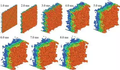
FIGURE 17.
Instantaneous images of TMZ visualized by the volume fraction isosurface YSF6 = 0.1, 0.3, 0.5, 0.7, and 0.9 from blue to orange at different times.
EVALUATION OF DIFFERENT SUBGRID‐SCALE STRESS MODELS
In large‐eddy simulation, the effect of small scales on large‐scale motions is represented by the SGS stress model. Most of the commonly used SGS models assume that the main function of subgrid scales is to remove energy from the large scales and dissipate it through the action of the viscous forces. But, as we know, in fact the energy is also transferred from the small scales to the large scales (backscatter) in a small and local range. The SGS turbulent dissipation, which is the work of SGS stress, represents the energy transfer between resolved and subgrid scales,
If it is negative, the subgrid scales remove energy from the resolved scales (forward scatter); if it is positive, they release energy to the resolved scales (backscatter). It is easy to see that the eddy viscosity models such as Smagorinsky model, Vreman model, etc. are absolutely dissipative.
Figure 18 shows the distribution of calculated SGS turbulent dissipation in streamwise direction for Smagorinsky and Vreman models and for AWE’s SF6 half‐height shock tube experiment [24] at two times [11]. The SGS dissipation of the Smagorinsky model is much greater than the Vreman model over 1.5 times; therefore, the dissipation is too great for the Smagorinsky SGS model. The SGS turbulent dissipations of the Vreman model (VM), the dynamic Smagorinsky model (DSM), and the stretched‐vortex model (SVM) based on a planar Richtmyer‐Meshkov instability with incident Mach number 1.2 are shown in Figure 19 [30]. Before the interfacial flow has developed to be turbulent completely, the dynamic and stretched‐vortex models have all predicted the energy backscatter, but the energy backscatter predicted by the dynamic model is larger and its range is wider. After reshock, the turbulent fluctuations are stronger extremely the turbulent dissipation also increases. The dynamic model’s dissipation is the highest, then followed by the Vreman model, and the stretched‐vortex model’s dissipation is the lowest. At the late time, the SGS dissipation of the dynamic and Vreman models is the same basically, and the dynamic model is also to be absolutely dissipative, yet the stretched‐vortex model is still able to predict the local phenomenon of energy backscatter in a small range. So, the dynamic model is poor in representing the energy backscatter. The Vreman and stretched‐vortex models are all robust, but the former is absolutely dissipative.
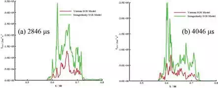
FIGURE 18.
Distribution of calculated SGS turbulent dissipation in a streamwise direction for Smagorinsky and Vreman models and for AWE’s SF6 half‐height shock tube experiment [24] at two times. Red line corresponding to the Vreman model, green line corresponding to the Smagorinsky model.
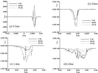
FIGURE 19.
Distribution of the SGS turbulent dissipation in a streamwise direction for the Vreman, dynamic Smagorinsky and stretched‐vortex models at four times.
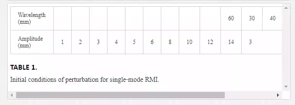
EFFECTS OF THE INITIAL CONDITIONS ON THE GROWTH OF SINGLE‐MODE RMI
single‐mode Richtmyer‐Meshkov instability without reshock [18]. The incident shock wave with Mach number 1.2 impacts the air/SF6 interface. The initial perturbation amplitude and wavelength are listed in Table First, we consider the effects of initial conditions of perturbation amplitude and wavelength on the growth of 1. The calculations are carried out in two dimensions, and the RMI does not develop into turbulent mixing completely. Figure 20 shows the effects of the initial perturbation amplitude on the growth of single‐mode RMI for the fixed initial perturbation wavelength λ0 = 60 mm. The perturbation amplitude (a) and growth rate (b) increase gradually with the increasing of initial amplitude. And when the initial amplitude is much larger, the growth of amplitude enters a linear stage earlier at the late times, and the growth rate remains a constant. The growth rate increases fast and reaches the highest peak at the early times. After the peak, the effect of compressibility is reduced and the flow nonlinearity starts to play a dominant role and causes the growth rate to decay with time. Figure 21 shows the effects of the initial perturbation wavelength on the growth of single‐mode RMI for the fixed initial perturbation amplitude a0 = 3 mm. The perturbation amplitude (a) and growth rate (b) reduce gradually at the early times and increase gradually at the late times with the increasing of initial wavelength. And when the initial perturbation strength (ration of initial amplitude to wavelength) is much smaller, the perturbation growth is mainly dependent on the initial perturbation amplitude and slightly dependent on the initial perturbation wavelength at the late times of RMI. The same conclusion can be obtained from three‐dimensional calculations.
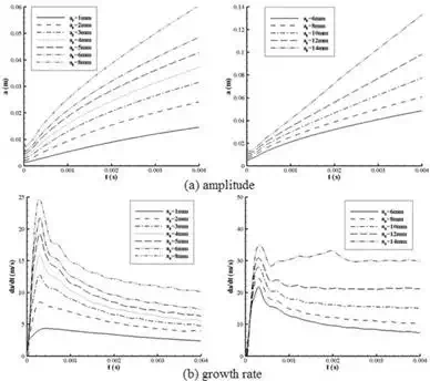
FIGURE 20.
Effects of the initial perturbation amplitude on the growth of single‐mode RMI for the fixed initial perturbation wavelength λ0 = 60 mm.
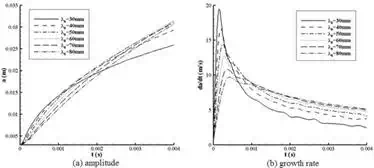
FIGURE 21.
Effects of the initial perturbation wavelength on the growth of single‐mode RMI for the fixed initial perturbation amplitude a0 = 3 mm.
EFFECTS OF THE INITIAL CONDITIONS ON THE GROWTH OF MULTI‐MODE RMI AND THE INDUCED TURBULENT MIXING
For the effects of three‐dimensional initial multi‐mode conditions, the case of Richtmyer‐Meshkov instability is same as the above Section 4.1. Table 2 lists the initial condition of perturbations, the perturbation strength (PS) is defined as the ratio of initial amplitude to wavelength. Turbulent kinetic energy K, dissipation rate ε, and enstrophy Ω are defined as follows [31]:
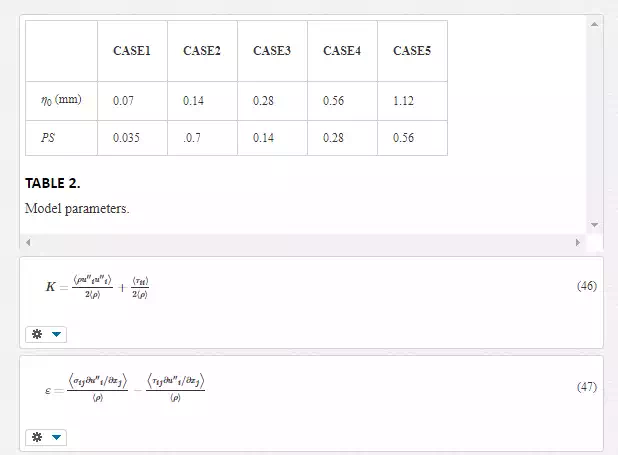
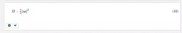
where u′′iu″i is the velocity fluctuation and 〈 〉 denotes the transverse plane‐average. For large‐eddy simulations, the turbulent kinetic energy and dissipation rate both include two parts named as the resolved‐scales (the first term on the right side of Eqs. (46) and (47)) and the subgrid‐scales (the second term on the right side of Eqs. (46) and (47)).
Figure 22 shows the growth history of TMZ width. Figures 23 and 24 show the time histories of the perk values of turbulent kinetic energy and enstrophy, respectively. For the larger initial perturbation strength, the TMZ grows faster, the turbulent kinetic energy is also larger or the turbulence strength is also stronger, the deposited vorticity is larger too. The development of turbulent mixing has a strong dependence on the initial conditions between the initial shock and the impingement of the first reflected rarefaction wave, after that the evolution of the turbulent mixing has lost the memory of the initial conditions.
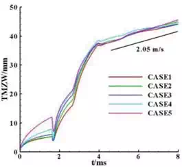
FIGURE 22.
Growth history of the TMZ width for different models
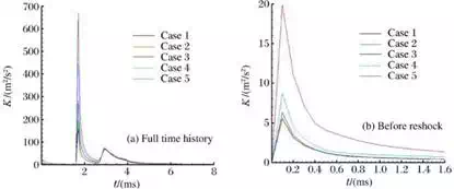
FIGURE 23.
History of turbulent kinetic energy for different models
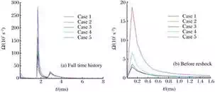
FIGURE 24.
History of enstrophy for different models
DYNAMIC CHARACTERS OF MULTI‐MODE RM INSTABILITY AND INDUCED TURBULENT MIXING
Figures 25–27 show the spatial profiles of the turbulent kinetic energy, dissipation rate and enstrophy along the motion direction of shock wave at different times before and after reshock individually. They all have a spatial profile similar to Gaussian distribution. The strongest turbulent intensity is located in the center of TMZ. Figures 28–30 show the temporal evolutions of the peak values of the turbulent kinetic energy, dissipation rate, and enstrophy in the spatial profiles, along with their fitted results, respectively. The turbulent kinetic energy, dissipation rate, and enstrophy decay gradually because of dissipation and diffusion. After the initial shock and before the reshock, the turbulent kinetic energy and enstrophy decay with time as a power law ;tθ except the dissipation rate which decays with time as an exponential law ;e−t/t∗e−t/t*. One reason is that the TMZ is not fully developed turbulence before reshock and the other reason is that the flow in TMZ is stronger anisotropic between the transverse direction and the axis direction. After reshock and the first reflected rarefaction wave, they all decay with time as the negative exponential law with the closed decay factors at the same stage, and be similar to the growth of TMZ width. And then, they all decay asymptotically due to no remarkable energy deposition. Therefore, the turbulent mixing behaves in a statistical self‐similar pattern. Figure 31 shows the one‐dimensional global energy spectra of three velocity components on a log‐log scale at three times. The energy spectra of two transverse components of velocity are too close, and there is a difference between transverse and axis components. The turbulent mixing flow is continuous anisotropic yet the anisotropy weakens gradually. That is to say, the development of the turbulent mixing presents a trend of isotropy.
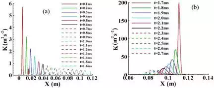
FIGURE 25.
Spatial profiles of the turbulent kinetic energy at different times. (a) Before reshock and (b) after reshock.
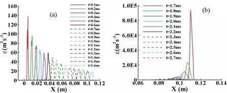
FIGURE 26.
Spatial profiles of the turbulent kinetic energy dissipation rate at different times. (a) Before reshock and (b) after reshock.
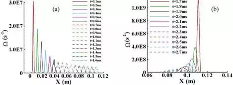
FIGURE 27.
Spatial profiles of the enstrophy at different times. (a) Before reshock and (b) after reshock.
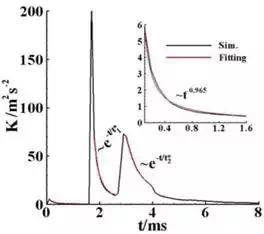
FIGURE 28.
Time history of the peak value of turbulent kinetic energy.
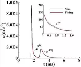
FIGURE 29.
Time history of the peak value of turbulent kinetic energy dissipation rate
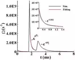
FIGURE 30.
Time history of the peak value of enstroph
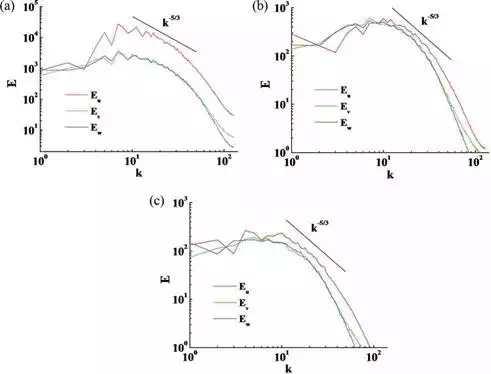
FIGURE 31.
One‐dimensional global energy spectra of three components of velocity on a log‐log scale.
NUMERICAL STUDY OF THE ELLIPTIC GAS CYLINDER INSTABILITY
Our group first performed the experimental and numerical investigations of the elliptic gas cylinder instability. As we know that the initial density distribution of the gas cylinder is hard to determine in the experiment, which can only give the one‐dimensional radial concentration distribution for circular gas cylinder as an approximate Gaussian function. Drawing to the experience on the one‐dimensional diffusive interfacial transition layer with finite thickness for circular gas cylinder, we constructed a two‐dimensional diffusive interfacial transition layer with finite thickness for elliptic gas cylinder through numerical simulation [32],
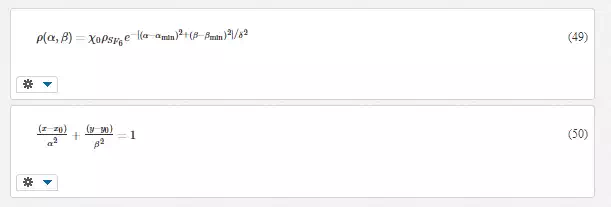
where x0 = y0 = 0, α ∈ [αmin, αmax], β ∈ [βmin, βmax], αmin = βmin = 1.0 × 10⁻⁵ mm, αmax = 6.30 mm, βmax = 2.30 mm, and δ = 6.16 mm. χ0 = 0.71 is the concentration of the elliptic center. The density distribution is plotted in Figure 32. The Mach number of air shock wave is 1.25. The simulations (see Figure 33) reproduce the elliptic gas cylinder instability experiment very well, they achieve to a good agreement qualitatively and quantitatively, some salient features of the vortex pairs are obtained clearly.
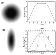
FIGURE 32.
Density images and distributions of the (a) circular and (b) elliptic SF6 gas cylinder initially constructed.
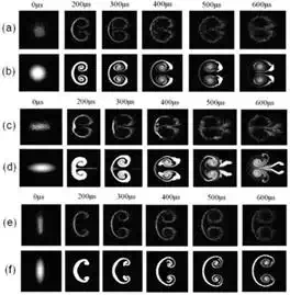
FIGURE 33.
Experimental evolution images and numerical simulation results by MVFT at t = 200, 300, 400, 500, and 600 µs, the experiments corresponding (a), (c), and (e), and the simulations corresponding (b), (d), and (f).
Figure 34 shows the vorticity at the center of the core and the distance between the two vortex cores of these two simulations. When the incident shock accelerates the elliptic gas cylinder along the major axis, the absolute vorticity in the vortex core |ωcore| is larger; but the distance between two vortex cores is larger when the incident shock accelerates the cylinder along the minor axis. So, the effect of convergence is stronger when the incident shock accelerates the elliptic gas cylinder along the major axis, for which the gas jet appears at the symmetry center.
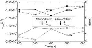
FIGURE 34.
Vorticity at the center of the cores and the distance between the two vortex cores from simulations.
FOUNDATION OF NEW RM INSTABILITY AND MECHANISM
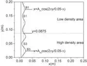
At present, the investigation for the Richtmyer‐Meshkov instability is performed in a uniform flow field. We first study the Richtmyer‐Meshkov instability and turbulent mixing in a nonuniform flow field by experiment and numerical simulations and find some new phenomena. Figure 35 shows the test section schematic of shock tube. The air shock wave with Mach number 1.27 accelerates the two‐mode sinusoidal air/SF6 interface (amplitude A01 = 5 m, A02 = 7.5 mm). The experimental Schlieren images (gray images in Figure 38) show the transmitted shock wave and the interface all incline which is different from the familiar RMI. We think this may be owing to the nonuniformity of flow field. Also, drawing to the experience on the diffusive interfacial transition layer of circular gas cylinder, we construct a nonuniform flow field with a Gaussian distribution of density along the direction perpendicular to the shock motion direction (as shown in Figure 36). The numerical result (shown in Figure 37) confirms this idea [12, 33, 34].
FIGURE 34.
Vorticity at the center of the cores and the distance between the two vortex cores from simulations.
FOUNDATION OF NEW RM INSTABILITY AND MECHANISM
At present, the investigation for the Richtmyer‐Meshkov instability is performed in a uniform flow field. We first study the Richtmyer‐Meshkov instability and turbulent mixing in a nonuniform flow field by experiment and numerical simulations and find some new phenomena. Figure 35 shows the test section schematic of shock tube. The air shock wave with Mach number 1.27 accelerates the two‐mode sinusoidal air/SF6 interface (amplitude A01 = 5 m, A02 = 7.5 mm). The experimental Schlieren images (gray images in Figure 38) show the transmitted shock wave and the interface all incline which is different from the familiar RMI. We think this may be owing to the nonuniformity of flow field. Also, drawing to the experience on the diffusive interfacial transition layer of circular gas cylinder, we construct a nonuniform flow field with a Gaussian distribution of density along the direction perpendicular to the shock motion direction (as shown in Figure 36). The numerical result (shown in Figure 37) confirms this idea [12, 33, 34].
Initial structure diagram in the shock tube.
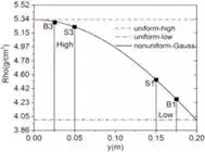
FIGURE 36.
Density profiles of nonuniform flows with Gaussian function and uniform flows in a vertical direction.
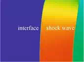
FIGURE 37.
Simulated density distribution in a nonuniform flow field by using Gaussian function.
Figure 38 shows the evolution of the interface and the propagation of the transmitted shock wave, the calculated results agree well with the experiment. Due to the nonuniform flow field of SF6 gas, the propagating velocity of transmitted shock wave in the upper part of shock tube is faster than in the bottom of shock tube, and it forms an oblique shock wave front and the interface. Figure 39 shows the shock front locations between experiment and numerical simulations, Figure 40 shows the perturbation amplitude of experiment, numerical simulation, and theories, they are in good agreement. Figure 41shows the calculated perturbation amplitude of RM instability for different modes in the initial uniform and nonuniform flow fields. As we can see that, at late times, the growth of small perturbation in a low‐density zone catches up and exceeds the large perturbation in a high‐density zone, which is opposite to the case of uniform flow field. Figure 42 shows the perturbation amplitudes of four different initial amplitudes 2.5, 5.0, 7.5, and 10 mm in low‐ and high‐density zones of nonuniform flow fields. It shows that the effect of initial amplitude on the growth of RM instability in the nonuniform flow field is different from the case of uniform one, which can be explained by the baroclinic vorticity shown in Figures 43 and 44, the baroclinic vorticity produced in the low‐density zone is larger than that in the high‐density zone.
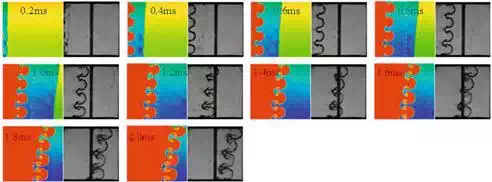
FIGURE 38.
Experimental schlieren photography images and numerical simulation results by MVFT2D at a certain time series (the sizes of the pictures are ones of the test window [0.038, 0.25 m] × [0.0, 0.2 m]).
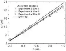
FIGURE 39.
Shock front locations of the experiment and calculated results on the three test lines.
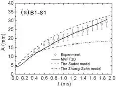
FIGURE 40.
Perturbation amplitudes of the experiment, simulation, and comparison with theories.
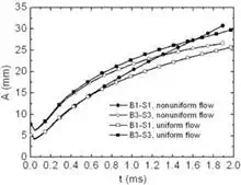
FIGURE 41.
Calculated perturbation amplitude of RM instability for different modes in the initial uniform and nonuniform flow fields.
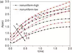
FIGURE 42.
Perturbation amplitudes of four different initial amplitude 2.5, 5.0, 7.5 and 10 mm in the low and high density zones of nonuniform flow field.
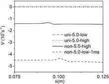
FIGURE 43.
Average vorticity when initial amplitude is 5.0 mm which is in the low and high density zones of nonuniform flow field at 1 ms.
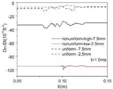
FIGURE 44.
Baroclinic vorticity in the uniform and nonuniform flow fields with the initial amplitude group (A01 = 2.5 mm,A02 = 7.5 mm) at 1.0 ms.
For the above investigations of RM instability in the nonuniform flow field, they are all without reshock. In the following section, we will study the effect of nonuniformity of flow field and the reshock on the RM instability. Here, we consider two kinds of nonuniformity: the nonuniform coefficient δ1 = 0.6162 m and δ2 = 0.4961 m. Figure 45 shows the density contour of the numerical simulated by MVFT at a time series, the left column with a uniform initial conditions, the middle column with a δ1 nonuniform Gaussian function, and the right column with a δ2 nonuniform Gaussian function. There is a significant difference between the uniform and reshock. Figure 46 shows the TMZ width of RM instability in the initial uniform and nonuniform flow fields. It points out that the growth of the TMZ width for the initial nonuniform flow field is greater than that for the uniform flow field, and the lesser the nonuniform coefficient, the higher the growth rate of TMZ width, but the difference for the nonuniform flows before reshock, but the difference decreases in evidence after three different flow configurations diminishes after reshock.
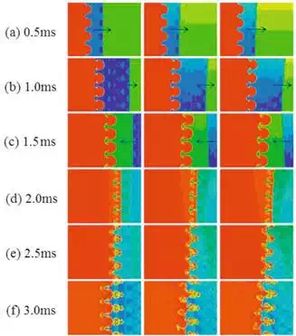
FIGURE 45.
Density contour of the numerical simulated by MVFT at a time series. The left column with a uniform initial condition, the middle column with a δ1 nonuniform Gaussian function, and the right column with a δ2 nonuniform Gaussian function. The small arrow denotes the direction of propagation of the shock wave fronts before reshock the interface
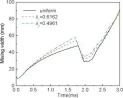
FIGURE 46.
TMZ width of RM instability in the initial uniform and nonuniform flow fields.
Prospect
Now, we investigated the Richtmyer‐Meshkov instability and the induced turbulent mixing in fluid flow by using large‐eddy simulation, but the turbulent mixing is a complicated three‐dimensional problem with multiple time‐space scales, and the more engineering applications involve the materials mixing with strength. So, the future work will be carried out in the following aspects: (a) the direct numerical simulations with high precision and high resolution on the platform of supercomputer, (b) the interface instability and turbulent materials mixing with strength, this may involve the material properties such as the deformation, fracture, melt, phase transition, material microstructures, etc., and it may make this problem to be more difficult.
Professor Jingsong Bai and Associate professor Tao Wang from the Institute of Fluid Physics, China Academy of Engineering Physics, People’s Republic of China and some other from the same institute should be thanked for the contributions and helps to these works, such as Prof. Ping Li, Dr. Liyong Zou, Kun Liu, Mr. Jinhong Liu, Min Zhong and Bing Wang, and Jiaxin Xiao.
The authors would like to thank the support from “Science Challenge Project” (no. TZ2016001), the National Natural Science Foundation of China (nos. 11372294, 11202195, 11072228, and 11532012), the Science Foundation of China Academy of Engineering Physics (nos. 2011B0202005, 2011A0201002, and 2008B0202011), and the Foundation of National Key Laboratory of Shock Wave and Detonation Physics (no. 9140C670301150C67290).