Numerical method

Simulations in the present study were all run using the commercial CFD code Ansys FLUENT. The DHRL methodology was implemented using the User-Defined Function subroutines available with that solver. Other turbulence models were all available as built-in modeling options in FLUENT. All of the test cases considered are incompressible, so the segregated pressure-based solver was used with the SIMPLE pressure-velocity coupling method. Second-order implicit (three-point backward difference) discretization was used for the unsteady term in all time-dependent simulations including HRL and LES. A second-order upwind, linear reconstruction scheme with a Least-Squares gradient computation and conventional slope limiting was used as the baseline discretization scheme for the convective terms in the momentum equations. Mass fluxes were computed using the momentum-weighted interpolation method of Rhie and Chow. For some of the test cases, a less dissipative bounded central differencing spatial discretization scheme based on the Normalized Variable Diagram was used to evaluate the influence of discretization scheme on the HRL results. A second-order centered discretization was used for the pressure gradient terms, and second-order central differencing was used for all diffusion terms.

Steady RANS simulations were run until a converged solution was obtained, with convergence determined based on stabilization of all flow variables to constant values as iterations increased, and a decrease in the L2 norm of all residuals by at least six orders of magnitude less from the initial value. For the hybrid RANS-LES (HRL) models, the converged steady-state RANS results were used as the initial conditions. The HRL model simulations were time-dependent and were run until a statistically steady-state flow field was obtained, as judged by time-averaged variables obtaining constant values with increasing time steps. The time-step size for unsteady simulations was selected to maintain maximum convective CFL number of approximately one, based on the smallest streamwise mesh dimension and the freestream velocity. For the time-dependent cases, the L2 norm of all residuals was verified to be reduced by at least three orders of magnitude during each time step. For both attached and separated flow test cases, an additional HRL simulation was run with the time-step size reduced by half, and results were compared to the default time step cases. No significant difference was observed for the resulting statistical quantities, so it was concluded that the use of a convective CFL number of approximately one is appropriate.

Attached turbulent flow test case

The selected attached flow test case is a fully developed turbulent channel flow, corresponding to the experimental study of Hoyas and Jimenez. Results for this case using the DHRL model were previously obtained using a pseudo-spectral solver and a combination of the Spalart-Allmaras one-equation model for the RANS component and the dynamic Smagorinsky model for the LES component. This paper investigates in more detail DHRL simulation using a general-purpose finite-volume flow solver.

The simulations were performed for the case of Reynolds number equal to 2003, where

u_τ is the wall friction velocity, δ is the channel half-height, and ν is the kinematic viscosity. The domain extent was 2πδ in the streamwise and πδ in the spanwise directions. Three different structured meshes were investigated, with streamwise × spanwise × wall-normal cell counts of 32 × 24 × 36 (Coarse), 64 × 48 × 72 (Medium), and 128 × 96 × 144 (Fine). The grid spacing was uniform in the streamwise and spanwise directions. Stretching was employed in the wall-normal direction so that the first near-wall cell centroid was located with y⁺ of 2, 1, and 0.5 for the Coarse, Medium, and Fine grids, respectively, and cells located at the channel centerline had aspect ratios of approximately unity.

Hybrid RANS-LES simulations were performed with three different models—the DHRL method described above, the original detached-eddy simulation (DES) model based on the Spalart-Allmaras RANS model, and the more recently proposed delayed detached-eddy simulation (DDES) model. The DHRL model combined the k-ω SST model as the RANS component and monotonically integrated LES (MILES) as the LES component. For comparison purposes, steady RANS simulations were obtained using k-ω SST model alone, and LES simulations were obtained using the MILES method. Results for all models were evaluated based on comparison with the available DNS data. Quantitative comparisons were made primarily for mean velocity and turbulent kinetic energy. Of particular interest was the effect of grid resolution level and discretization scheme for the different modeling approaches investigated. Unless otherwise noted, all results shown are plane-averaged, though all statistical quantities showed little variation in the streamwise and spanwise directions once the simulation had run sufficiently long for a stationary state to be reached.

Figure 1 shows the mean velocity profile predicted by each of the models on the Coarse, Medium, and Fine grids. Note that the results with the SST model are only shown for the Coarse grid, since no noticeable differences were observed between that and the two finer grids. The MILES results are only shown for the Medium and Fine grids, since the results on the Coarse grids were comparable to laminar flow, and dramatically overpredicted the velocity in the middle portion of the channel. In fact, it is apparent from Figure 1 (b) that even results on the Medium grid are qualitatively incorrect, and only on the Fine grid does the characteristic log-layer behavior begin to be observed, though mean velocity of it is still significantly overpredicted.

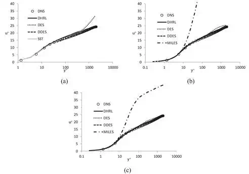
Figure 1.

Mean velocity profiles for turbulent channel flow test case using different turbulence models: (a) Coarse mesh; (b) Medium mesh; (c) Fine mesh.

For the Coarse grid, the SST, DDES, and DHRL models all show qualitative agreement with the DNS data, with the DDES model showing the best agreement, and both the SST and DHRL models showing a similar, slight overprediction in the log-layer region. The DES model shows the characteristic overshoot that has previously been noted in the literature, which is due to the performance of the model in the transition region between the (near-wall) RANS zone and the far-field (LES) region in the middle of the channel. As the grid is refined (Figure 1 (b, c)), the DES results agree more closely with the DNS data, and for the Fine grid, the log-layer mismatch is much smaller, though still apparent.

For all three grid sizes, the DDES model obtained a numerically steady-state result, effectively operating as a pure RANS model. This is not surprising, since the goal of the Delayed DES formulation is to inhibit the development of LES behavior in attached flow regions, while allowing its development in separated flow regions. As a consequence, the DDES mean velocity results were limited to a Spalart-Allmaras model equivalent, which is in good agreement with the reference data.

The predicted turbulent kinetic energy (k) profiles for the hybrid RANS-LES models are shown in Figure 2. Since the DDES model returned a steady RANS solution, no result is plotted. For the DHRL model, both resolved turbulence and total (resolved + modeled) turbulence is shown, where the totl k is computed as:

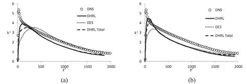
Figure 2.

Turbulent kinetic energy (k) profiles for turbulent channel flow test case comparing results with DES and DHRL models: (a) Medium mesh; (b) Fine mesh. For DHRL, both resolved k and total k (resolved + modeled contributions) are shown.

For both the DES and DHRL models, the overall trends are correctly predicted, with a peak near the wall and decay to a minimum value at the channel centerline. Both models tend to underpredict the peak value of k near the wall as well as predicting the location of the peak to be too far from the wall, and for the Fine grid case show an underprediction throughout the channel. The DES result shows nontrivial sensitivity to the mesh refinement level, and surprisingly shows better agreement throughout most of the channel on the Coarse grid than on the Fine grid. The DHRL model shows relatively little dependence on the mesh resolution level, except for an improvement in the near-wall prediction as the grid is refined (as does the DES model).

The mesh sensitivity is further highlighted in Figure 3, which shows the change in the mean velocity profiles for each model as the mesh is refined from 27,648 total cells (Coarse) to 1,769,472 cells (Fine). For the DES model (Figure 3 (a)), the improvement with increasing mesh resolution is apparent, as the characteristic overshoot becomes smaller. The DDES model is not shown since it yielded a steady-state result that was insensitive to mesh refinement level for the grids considered here. The DHRL model (Figure 3 (b)) shows very little sensitivity to grid refinement level and shows better agreement with the DNS data than the DES model for all refinement levels. Also shown in Figure 3 (b) are the steady RANS results from the SST model, which is the RANS component for the DHRL hybridization. The results from DHRL agree quite closely with the SST for all mesh refinement levels, despite the fact that a significant portion of the turbulent kinetic energy is resolved as unsteady velocity fluctuations (Figure 2) in contrast to the steady SST result.

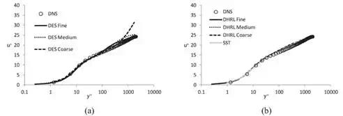
Figure 3.

Effect of grid resolution on predicted mean velocity profiles for DES (a) and DHRL (b) models.

The effect of the choice of discretization scheme (second-order upwind versus NVD-based Bounded Central Difference) for the convection term is shown in Figure 4, for both the DES and DHRL models. While the BCD scheme has been shown to significantly reduce numerical dissipation on structured meshes [35, 36], the effect on the mean flowfield using hybrid RANS-LES models was found to be insignificant. For the DES model, as the numerical dissipation increases, the local shear stresses decrease in magnitude, resulting in lower overall magnitudes of the eddy viscosity. This decrease in model eddy viscosity helps to compensate for the higher numerical viscosity of the second-order upwind scheme. For the DHRL model, a similar effect occurs. As seen in Eq. (10), the blending coefficient α responds to changes in the resolved flowfield to adjust the RANS contribution accordingly.

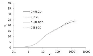
Figure 4.

Effect of discretization scheme (second-order upwind vs. bounded central difference) on predicted mean velocity profiles for DES and DHRL models.

The underlying method by which the DHRL model operates is highlighted in Figure 5, showing the distribution of the blending parameter α through the channel for all three grids investigated. Recalling that α = 0 corresponds to a pure RANS mode and α = 1 corresponds to a pure LES mode, it is apparent that both the Medium and Fine grid cases have a significant portion of the channel, up to about y+ = 1000, for which the model operates as pure MILES. The MILES region extends further toward the wall for the Fine grid case (y+ ~ 100) than for the Medium grid case (y+ ~ 300). In the near-wall region, α → 0 as y→0 and the RANS model is recovered. Likewise, near the channel centerline (y+ > 1000), α < 1 and some portion of the RANS model stress is introduced into the momentum equations. The behavior of the Coarse grid case is quite different. Since the mesh is too coarse to resolve a significant level of turbulent production, the value of α is quite low throughout the channel, and a significant portion of the RANS model stress is introduced. As seen in Figure 1 (a), the effect is to minimize overshoot of the mean velocity profile in the middle portion of the channel and recover a result close to the steady RANS SST result.

.

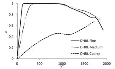
FIGURE 5.

Variation of DHRL blending parameter (α) across the channel for three different mesh sizes.

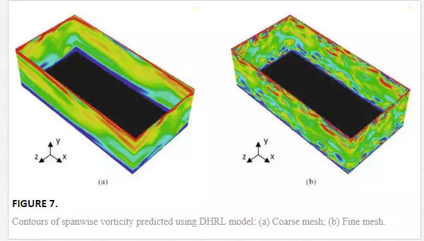
Figures 6 and 7 illustrate some of the features of the resolved velocity field in the hybrid RANS-LES simulations. Figure 6 shows isosurfaces of Q-criterion on the Fine grid, for both the DES and DHRL models, to highlight the presence of vortical turbulent structures. Such structures are visible for both models; however, for an equivalent value of Q-criterion, the structures predicted by the DHRL model are more prevalent and of a smaller scale than those predicted by the DES model. This was found to be consistently true for all cases. The reason is that the DHRL model operates in a MILES mode with respect to the fluctuating velocity field and as such the dissipation of small-scale turbulent features is less than with the DES model. Figure 7 shows qualitatively the effect of mesh refinement on the resolution of the fluctuating velocity field using the DHRL model by showing contours of the spanwise vorticity on the periodic boundary planes. It is apparent that for the Fine grid (Figure 7 (b)), a significant portion of the turbulent spectrum is resolved, similar to the Q-criterion contours in Figure 6 (b). However, for the Coarse grid (Figure 7 (a)), only large-scale, low-frequency fluctuations are present in the flow. It is this lack of resolution of the turbulence field that results in the decrease of the blending parameter α (Figure 5) in the Coarse grid case, and the introduction of a relatively large RANS stress contribution into the momentum equations.

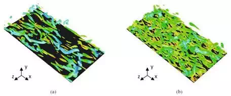
FIGURE 6.

Isosurfaces of Q-criterion showing resolved turbulent structures on the Fine grid: (a) DES and (b) DHRL.

Separated turbulent flow test case

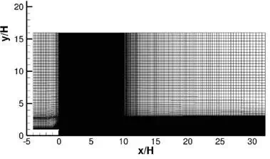
The separated flow test case is the backward facing step flow matching the experimental study of Driver and Seegmiller [26], which is a commonly used benchmark case for turbulence model verification and validation. Two different three-dimensional meshes were created using the commercial meshing tool Ansys GAMBIT^® in order to evaluate grid sensitivity issues common to most current HRL models [15], for example, the delay of instability and breakdown of separated shear layers. For both grids, the computational domain size extended from 4 step heights (H) upstream of the step to 32H downstream of the step, 16H vertically from the wall downstream of the step, and 6H total in the spanwise direction. A structured multiblock mesh was generated, with a baseline Coarse mesh containing 744,960 total cells, and a Fine mesh containing 7,946,400 total cells. An average y+ value less than one was enforced to satisfy the recommended y+ requirements for the RANS turbulence model and for accurate HRL modeling. Nearly isotropic quadrilateral cells were used in the LES region (from x/H = 0.0 to 10.0) for maximum accuracy. A 2D planar slice of the Fine mesh is shown for illustrative purposes in Figure 8

Simulations were performed using the DHRL, DDES, and SST k-ω models, with all simulation parameters and boundary conditions matching the experimental study. Profiles of inlet flow variables including mean inflow velocity, turbulent kinetic energy, and specific dissipation rate for the DHRL and RANS model simulations, and modified eddy viscosity for the DDES model simulation were created to match the distributions in the experimental data. For the spanwise boundaries, a periodic boundary condition was applied in the transient HRL simulations, and a symmetry boundary condition was used for the steady RANS simulation.

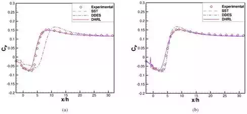
Figure 9 shows the spanwise-averaged mean wall static pressure distribution for both the Coarse mesh and the Fine mesh, respectively, using three different turbulence models. In the recirculation region (x/H > 0), the Coarse mesh results shown in Figure 9 (a) indicate that both the DHRL and RANS computations predict a smooth pressure decrease and resolve the negative peak pressure with reasonable accuracy compared with the experimental data. The DDES results in contrast show overprediction of the pressure decrease and an offset in the location of negative peak pressure. The pressure rise predicted by both the DHRL and RANS models in the separated flow region shows similar behavior to the experimental results, but the wall pressure in the DDES computation shows a delayed pressure recovery. The pressure distribution after flow reattachment is similar to the experimental results for all simulations, except for a small overprediction by the DDES model in the region 10 < x/H < 16. Figure 9 (b) shows that the Fine mesh computations compare reasonably well with the experimental data for all models used. Simulations using the Fine mesh show a substantial improvement relative to the Coarse mesh for the DDES model. The differences underscore the mesh sensitivity inherent in DDES. In contrast, the Coarse and Fine mesh results using the DHRL model are similar, indicating that the DHRL

model is relatively insensitive to mesh resolution, which agrees with the results from the attached flow test case above.

FIGURE 9.

Static pressure distribution on wall downstream of step: (a) Coarse mesh; (b) Fine mesh.

Figure 10 shows the spanwise-averaged mean wall skin friction distribution on both the Coarse mesh and Fine mesh. Figure 10 (a) indicates that the wall skin friction result on the Coarse grid in the separated flow region agrees closely with the experimental data for both the DHRL model and the RANS model. In particular, the negative peak Cf values are quite close to the experimental result. In contrast, the DDES model shows an overprediction of the size of the flow separation region along with an overprediction of skin friction. The reattachment point was determined in the experiments using a linear interpolation of the oil-flow laser skin-friction measurements and was found to be x/H = 6.38 [26]. The DHRL model results show an early prediction of flow reattachment and a reattachment point of approximately x/H = 5.60, an underprediction of 9%. The RANS model predicts the flow reattachment location at x/H = 6.30, which is closer to the experimental measurements. The DDES results show a delayed flow reattachment at x/H = 9.23. The grid is too coarse for the DDES model to accurately resolve the Reynolds stress contribution in either LES or RANS mode, leading to the delay in flow reattachment. The skin friction is predicted reasonably well by the DHRL model downstream of the reattachment point. The RANS model accurately predicts skin friction immediately downstream of the reattachment point but shows an underprediction in the region farther downstream. The differences in the DHRL model prediction, as compared to the SST model, can be attributed to the presence of resolved unsteady turbulent fluctuations in the flow that lead to more rapid mixing of the separated shear layer and transport of momentum in the wall-normal direction. This is also clearly seen in the mean velocity and turbulent kinetic energy profiles shown below.

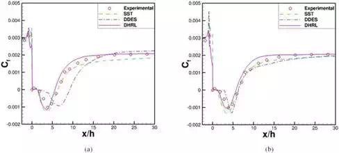
FIGURE 10.

Skin friction distribution on wall downstream of step: (a) Coarse mesh; (b) Fine mesh.

The predicted skin-friction distribution for the Fine mesh, shown in Figure 10 (b), indicates that results with all three models agree reasonably well with the experimental data. However, with regard to mesh sensitivity, some models show quantitative or even qualitative differences between the Coarse and Fine meshes. The DHRL model predictions are closest to being mesh insensitive, as the Cf calculations for both meshes are quite similar. The reattachment location (x/H = 5.70) calculated using the Fine mesh is less than 2% different than the result on the Coarse mesh. The RANS model predictions for both the Coarse and Fine meshes show very close agreement with one another in all regions, including the separation point. This is similar to the attached flow results above, for which the steady RANS results were effectively mesh independent. In contrast, a significant level of mesh sensitivity is shown by the DDES model predictions. Skin friction over most of the downstream wall shows significant differences between the Coarse and Fine grid results. Mesh refinement significantly improves the prediction of reattachment point (x/H = 6.31) for the DDES model.

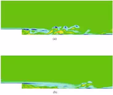
Previous studies have shown that DDES model predictions have reported delayed shear layer breakup and limited resolution of the Reynolds stresses in separated flow regions, particularly on coarse grids. One key advantage of the DHRL model is that it inherently addresses these potential problems. Figure 11 shows contours of instantaneous spanwise vorticity (z-vorticity) obtained from the DHRL and DDES model simulations, respectively, on the Coarse mesh. The DHRL model results indicate a better ability to resolve turbulent eddies in the separated shear layer and a more obvious breakup and transition to LES mode than the DDES model. The relatively poor predictions of wall static pressure and skin friction predictions by the DDES model shown above are partly explained by these results. Figure 12 shows the contours of instantaneous spanwise vorticity (z-vorticity) on the Fine mesh for both models. DHRL and DDES are both able to resolve turbulent scales in the separation region and as a result are able to provide reasonably accurate prediction of Cp and Cf. With regard to mesh sensitivity, the DHRL model contours are similar on both the Coarse and Fine mesh computations except for the increased resolution of small scales on the Fine mesh. The DDES model contours, in contrast, show even qualitative differences between results on the Coarse and Fine meshes. Figure 13 shows the spanwise vorticity (z-vorticity) contours predicted by the RANS simulations on the Coarse and Fine meshes, respectively. It is apparent that no turbulent scales are directly resolved, as expected. Rather, the effect of all turbulent scales on the mean flow is included via the eddy-viscosity term.

FIGURE 11.

Contours of instantaneous resolved z-vorticity for the Coarse mesh simulations: (a) DHRL; (b) DDES.

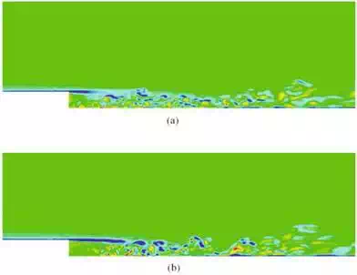
FIGURE 12.

Contours of instantaneous resolved z-vorticity for the Fine mesh simulations: (a) DHRL; (b) DDES.

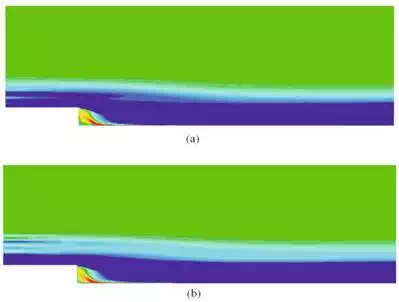
FIGURE 13.

Contours of instantaneous resolved z-vorticity using RANS model: (a) Coarse mesh; (b) Fine mesh.

In order to minimize the dissipation errors due to the numerical method, low dissipation schemes are generally used for convective term discretization in LES and HRL simulations. The bounded central differencing (BCD) [35] scheme is an example of a low-dissipation scheme developed to provide stable results on both structured and unstructured grids. Fine mesh simulations using the BCD scheme were performed along with baseline second-order upwind simulations to investigate the effect of discretization on the HRL model results. Figure 14 shows the distribution of pressure in the streamwise direction, obtained using the Fine mesh. Very little difference due to discretization scheme is observed for the DHRL results. The DDES simulations, in contrast, show more sensitivity to the scheme, with the BCD discretization method producing a slightly overpredicted negative Cp peak and a delayed pressure recovery relative to the second-order upwind results.

FIGURE 14.

Static pressure distribution on downstream bottom wall comparing results with BCD and second-order upwind discretization scheme on the Fine mesh.

Figure 15 shows skin friction predictions on the Fine mesh for DHRL and DDES using both discretization schemes. Again, there is little difference in DHRL simulations due to the numerical scheme, though slightly better agreement with experiments is observed in the BCD scheme predictions just downstream of the reattachment location. The reattachment point (x/H = 5.75) for the DHRL with BCD scheme is close to the predicted reattachment with the upwind scheme (x/H = 5.70). For the DDES model, the BCD scheme results show a streamwise offset for the Cf prediction in the separated flow region compared to the upwind scheme. The BCD scheme results also show a significantly delayed reattachment point (x/H = 6.80) relative to the upwind scheme (x/H = 6.31). To summarize, the effect of discretization scheme in the DHRL simulations appears to be minimal, with a slight improvement in the results when using the BCD scheme. The use of the BCD scheme for the DDES simulations appears to result in slightly less agreement with experimental data, which is surprising. The apparent reason for this behavior may be the violation of the convection boundedness criterion of the BCD method due to the very low sub-grid scale turbulent diffusivity produced by the DDES model simulations.

FIGURE 15.

Skin friction distribution on downstream bottom wall comparing results with BCD and second-order upwind discretization scheme on the Fine mesh.

Figure 16 shows mean streamwise velocity profiles at several streamwise measurement stations for simulations using the Fine mesh. In the separated flow region (stations x/H = 1.0, 1.5, 2.0, and 3.0), the profiles clearly show that characteristics including boundary layer growth and size of the separation bubble in the wall normal direction are well resolved by both the DHRL and RANS simulations in comparison to the experimental measurements. The DDES simulation shows a small underprediction of the negative velocity peak in the near wall region and an overprediction of the size of the separation bubble. Simulations using each of the models show good agreement with the experimental data far from the wall. Immediately upstream of the reattachment point (station x/H = 5.0), DHRL and RANS results show reasonably good agreement with the data in terms of the negative velocity peak and separation-bubble size, but the DDES model somewhat overpredicts the flow behavior. It is apparent that in the separated flow region near the wall, the DHRL simulation shows nearly RANS-like behavior, which is expected since the DHRL model tends to limit to the RANS result close to the wall unless the grid is highly refined. It is interesting to note that the experimental velocity profile at station x/H = 6.0 clearly shows that the flow has reattached, which is early relative to the experimentally determined reattachment location of x/H = 6.38 based on the oil-flow laser skin-friction measurements [26]. The reason for this apparent discrepancy in the experimental data is not clear. The DHRL results also predict reattached flow at station x/H =6.0, while the RANS and DDES simulations show separated flow. Farther downstream (x/H = 7.0), all models clearly show not only reattached flow but also an underprediction of the velocity very close to the wall. In the wake recovery region (x/H = 16.0 and 20.0), the two HRL models show good agreement with the experimental data while the RANS model results show an underprediction in the rate of wake recovery, presumably due to lower predicted levels of turbulent mixing.

FIGURE 16.

Predicted (Fine mesh) and measured mean velocity profiles at measurement stations downstream of the step. (a) x/H = 1.0. (b) x/H = 1.5. (c) x/H = 2.0. (d) x/H = 3.0. (e) x/H = 5.0. (f) x/H = 6.0. (g) x/H = 7.0. (h) x/H = 16.0. (i) x/H = 20.0.

Figure 17 shows computed turbulent kinetic energy profiles (normalized by square of mean inlet velocity) obtained for the Fine mesh simulations, compared with experimental data, at the measurement stations identical to those used to compare the mean velocity profiles. In the separated shear layer just downstream of the step at x/H = 1.0, DHRL results show the sudden rise in turbulent kinetic energy seen in the experimental data, indicating relatively rapid breakup of the shear layer characteristic of DHRL simulations. In contrast, the DDES model results show a relatively small peak in turbulent kinetic energy, which is characteristic of the more delayed shear layer break up characteristic of that model. This is also reflected in the delayed mixing of mean momentum shown at the same location in Figure 16. RANS model results show a relatively rapid increase in modeled turbulent kinetic energy downstream of flow separation. Both the DHRL and RANS results show a steady increase in turbulent kinetic energy similar to the experimental data up to station x/H = 5.0. The DDES simulation shows a relatively slow increase at stations x/H = 1.5 and 2.0, but a more rapid increase at x/H = 5.0, characteristic of a delayed but sudden breakup of the shear layer. Near the reattachment location at stations x/H = 6.0 and 7.0, the computed turbulent kinetic energy profiles decay similar to the experimental results, but the peak value of turbulent kinetic energy is underpredicted by the DHRL and RANS models results and significantly overpredicted by the DDES results. Farther downstream (stations x/H = 16.0 and 20.0), results obtained with all three models show qualitative agreement with the experimental data.

FIGURE 17.

Predicted (Fine mesh) and measured turbulent kinetic energy profiles at measurement stations downstream of the step. (a) x/H = 1.0. (b) x/H = 1.5. (c) x/H = 2.0. (d) x/H = 3.0. (e) x/H = 5.0. (f) x/H = 6.0. (g) x/H = 7.0. (h) x/H = 16.0. (i) x/H = 20.0.

Summary and conclusions

The recently proposed dynamic hybrid RANS/LES modeling framework (DHRL) has been investigated for two test cases, turbulent channel flow and flow over a backward facing step, in order to investigate the capability of the model to accurately predict both attached and separated turbulent flows. The test cases elucidated the behavior of the DHRL model in comparison with a more traditional hybrid RANS-LES model, including model response to mesh refinement level and changes in discretization scheme.

For the channel flow test case, the DES and DHRL models showed significant resolved velocity fluctuations for all mesh refinement levels and for both discretization schemes, on the order of the turbulence levels in the reference DNS data. In contrast, the DDES model yielded a steady RANS-type solution, which is consistent with its intended performance. The DES model exhibited the well-known log-layer mismatch in the mean velocity, which was significantly reduced for the DHRL model. Furthermore, the DES model showed significant mesh dependence, with results improving as the mesh was refined, as expected. The DHRL model showed almost no mesh sensitivity with regard to the mean flow results, although the resolved turbulent kinetic energy levels, as well as the range of resolved scales of fluctuating motion, increased with increasing mesh refinement. The DDES model and SST models showed no mesh dependence due to the fact that each yielded a steady-state result. Both the DES and DHRL models showed almost no sensitivity to discretization scheme for the attached flow case.

For the backward facing step test case, the DHRL results showed rapid breakdown of the shear layer from RANS to LES type flow even for the Coarse mesh simulations, and relatively small differences in results on both the Coarse and Fine meshes, as well as for two different discretization schemes. The DDES model results showed a delayed breakdown of the shear layer and substantial mesh dependence, as well as nontrivial dependence of the results on the discretization scheme. The mean flow results predicted using the DHRL model were similar to the SST model results in the separated flow region, but showed improved prediction downstream of the reattachment point. The DHRL results were also comparable to SST results and superior to DDES results in terms of predicted turbulent kinetic energy downstream of the step, although it should be noted that for the SST model turbulence was completely modeled while for the DHRL model turbulent kinetic energy was resolved as unsteady velocity fluctuations. A key benefit to the DHRL model is the potential to effectively address grid dependence issues present for most currently used HRL models in predictions of the mean flow, while providing for increasing resolution of unsteady turbulence fluctuations while operating in LES mode as the grid size is reduced.

Overall, the results indicate that the DHRL model performs as designed. The attached flow case demonstrates a smooth variation between the RANS and LES zones, perpendicular to the flow direction, controlled by the model blending parameter α. Likewise, the separated flow case showed a similar behavior, with transition between RANS and LES regions occurring in the streamwise and wall-normal directions. The lack of explicit grid dependence in the DHRL model terms resulted in minimal grid dependence of the mean flow results, in contrast with the DES and DDES models. Furthermore, the DHRL model was shown to agree closely with the RANS component (SST) results for the attached flow case, while resolving significant levels of turbulent fluctuations in the boundary layer, at least on well-refined grids. Results indicate that the DHRL model may provide a more flexible and universal method for hybrid RANS-LES than existing standalone models.