Model formulation

The DHRL model formulation is summarized in this section. Readers are referred to Bhushan and Walters [27] for a more detailed description. Other models, including DES, DDES, and SST k-ω, are also summarized since they are used to perform companion simulations, and the results are compared with DHRL. In addition, the SST k-ω model is used as the RANS component of the DHRL model, while MILES is used as the LES component. The models used here were chosen for comparison purposes because they are widely used examples of HRL and RANS, respectively. Since they have been previously thoroughly documented, only a brief description and appropriate references are provided in Subsections 2.2–2.5.

DYNAMIC HYBRID RANS-LES (DHRL) METHODOLOGY

The description of the DHRL model presented here focuses on single-phase, incompressible, Newtonian flow with no body forces. Extension to compressible flow or flows with gravitational effects is straightforward. First, applying an (undefined) filtering operation to the momentum equation results in:

where ui and uˆiûi are the instantaneous and filtered velocity, respectively. The last term on the right-hand side represents the turbulent stress, which corresponds in general to any residual stress tensor obtained from either Reynolds averaging or filtering. This can be expressed as follows:

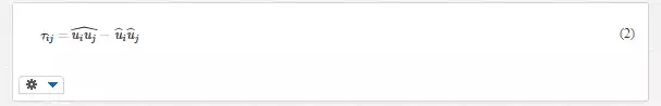
The turbulent stress term must be modeled in order to close the filtered momentum equation.

Most hybrid RANS-LES models, including the commonly used DES model, use a single scalar variable in the filtered momentum equation to model the turbulent stress using the Boussinesq hypothesis. This term is denoted as the eddy viscosity, and in theory obtains a value appropriate for a modeled Reynolds stress in the RANS region (typically near the wall) and a value appropriate for a modeled subgrid stress in the LES region (typically far from the wall).

As discussed above, blending the effects of ensemble-averaged velocity fields (Reynolds stress) and spatially filtered velocity fields (subgrid stress) using a single scalar variable introduces ambiguity into the model. The DHRL modeling methodology seeks to avoid this ambiguity. The model development begins with decomposition of the velocity field in such a way that the effects of ensemble-averaged velocity fields and spatially filtered velocity fields retain a distinct separation in the transitional or “gray” zones.

First is introduced a simulation-specific decomposition for the instantaneous velocity (ui):

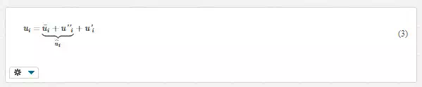
where uˆiûi is the velocity resolved in the simulation, ūi is the mean (Reynolds-averaged) velocity, u″i is the resolved fluctuating velocity, and u′i is the unresolved or modeled fluctuating velocity. The Reynolds-averaged velocity and resolved fluctuating velocity can be obtained directly from the simulation. The modeled fluctuating velocity is defined using the turbulent stress term. Substitution of the decomposed instantaneous velocity (ui) in Eq. (3) into Eq. (2), along with the assumption that resolved and unresolved velocity fluctuations are uncorrelated, yields the following expression for the residual stress:

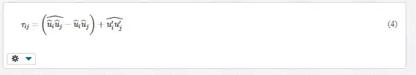
The scale similarity concept can be used to model both of the terms on the right-hand side of Eq. (4). The result is an expression for the subfilter stress term as:

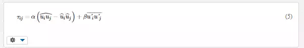
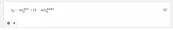
The first (both parts inside parenthesis) and the second terms on the right-hand side of Eq. (5) can be modeled as linear functions of the subgrid stress (SGS) and Reynolds stress, respectively. The SGS and Reynolds stresses can be obtained from any suitable SGS and RANS model. The proportionality constants α and β can be both spatially and temporally varying, but are assumed to be complementary, such that the residual stress term can be expressed as a weighted average of both the SGS and RANS stress as follows:

To determine the value of the blending coefficient α, a secondary filtering operation is applied, conceptually similar to the method of Lilly for dynamic model coefficient evaluation for subgrid stress modeling. Based on the following assumptions:

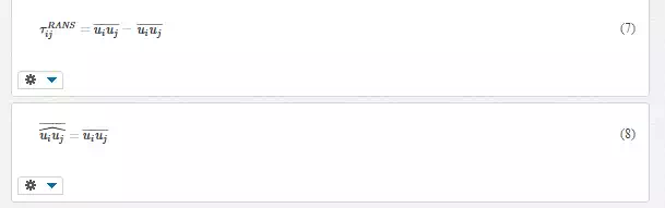
the Reynolds-averaging operation can be applied to Eq. (2) as a secondary filter and combined with Eq. (7) to yield:

:

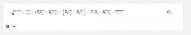
The Reynolds-averaged form of Eq. (6) is combined with Eq. (9) to eliminate τij¯¯¯¯. The scalar product of the result with the mean (Reynolds-averaged) strain rate yields the expression

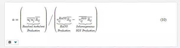
The local value of the coefficient α is determined based on the relative contribution to turbulence production by the resolved scales, the mean (Reynolds-averaged) component of the subgrid model stress, and the RANS model stress. For stability, the value of α is limited in practice to lie between 0 and 1. Eq. (10) shows that the value of α becomes zero in regions with no resolved fluctuations, i.e., numerically steady-state flow. In those regions, therefore, a pure RANS model is recovered. In regions for which turbulence production by resolved velocity fluctuations is significant, the RANS stress contribution decreases, and an LES subgrid stress contribution appears in the momentum equation. This ensures a smooth variation of turbulent production through the transition between RANS and LES. If the resolved turbulent production in any region is sufficiently large, α increases to a value of 1, and a pure LES model is recovered.

One final key aspect of the DHRL methodology is the manner in which the RANS model component is computed. In contrast to most other hybrid methods, the DHRL approach computes the RANS terms based only on the Reynolds-averaged flowfield. For stationary flows, the velocity field used to compute all RANS terms can be obtained from a time-averaging operation that runs concurrent with the simulations. Other appropriate averaging methods can be adopted for nonstationary flows. For the current study, stationary flows are considered, and the RANS model is computed using the time-averaged flowfield in all of the turbulence model terms.

Detached-eddy simulation (DES)

The DES model is based on the one-equation eddy-viscosity RANS model developed by Spalart and Allmaras (SA), which has been used extensively in applied CFD analysis. The SA model includes one additional transport equation for an eddy-viscosity variable, ν˜

. The transport equation includes terms for diffusive transport, production, and destruction, where the latter is given in simplified form as follows:

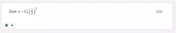
where C_d is a variable model coefficient and d is the distance to the nearest wall. The wall distance also appears in other model coefficients.

The DES model replaces the wall distance with an effective length scale, d˜

, that is a function of both wall distance and local mesh size:

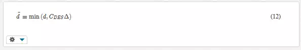
where ∆ is the local characteristic mesh spacing and C_DES is a model constant. The effect of the modification is to increase destruction of ν˜ in regions with Fine mesh, allowing the development of resolved turbulent fluctuations, while recovering the original SA RANS formulation in regions with large mesh spacing. The reader is referred to for further details.

Delayed detached-eddy simulation (DDES)

The DDES model was proposed as a modification to the baseline DES model in order to address the issue of grid-induced premature switching to the LES mode in attached boundary layers. This anomalous activation of LES mode occurs in the DES model when a highly refined grid is used. In contrast to the baseline DES model, DDES redefines the length scale such that it depends on both the local grid size as well as the eddy viscosity:

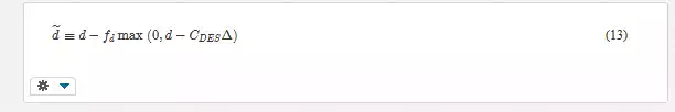
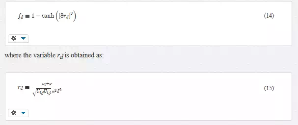
The function f_d recovers a value of zero inside the boundary layer, ensuring that the RANS mode is activated; however, the value of f_d limits to one outside the boundary layer, thus recovering the underlying DES mode. The functional form of f_d is

Shear-stress transport (SST) k-ω

The SST k-ω model proposed by Menter is conceptually based on the transport of the principal shear stress and was developed to improve prediction of flows with adverse pressure gradients. It has been used for a large number of practical RANS CFD simulations of complex turbulent flows. In the SST model, the eddy viscosity from the baseline k-ω model is modified within the framework of the SST model as follows:

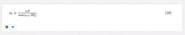
where F₂ is a blending function, a₁ is a constant, and S represents an invariant measure of the strain rate magnitude. F₂ recovers a value of one in attached boundary layers, and a value of zero in free shear layers. The model improves prediction in adverse pressure gradient boundary layers by ensuring that production of turbulent kinetic energy is larger than dissipation.

Two transport equations are adopted in the SST model, one for the turbulent kinetic energy (k) and one for the specific turbulence dissipation rate (ω):

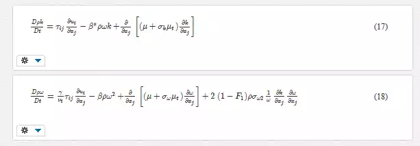
The function F₁ plays a similar role as the blending function F₂, acting as an indicator variable for near-wall and farfield regions of the flow. Near the wall, F₁ = 1, and the k-ω model form is obtained. In farfield regions, F₁ = 0 and the model behaves similar to a k-ε model. Refer for further model details. For the DHRL model used in the present study, the SST model was used as the RANS component.

Monotonically integrated large eddy simulation (MILES)

subgrid stress is assumed to be accurately approximated by the dissipation inherent in the discretization error for the convective terms. For upwind-biased schemes in particular, the numerical MILES refers to an approach for implicit LES first documented by Boris et al. for which the error can be shown mathematically to be similar in form to an explicit eddy-viscosity model for such an approach, and several studies have been documented in the literature in which practical LES solutions have been successfully obtained. For the present study, the MILES method is used for the reference LES simulations and also as the LES component in the DHRL implementation. Two different convective discretization schemes are used (these are discussed below). Both schemes are designed to preserve monotonicity through upwinding and flux limiting, which is appropriate for a MILES approach.