Sea Level Changes Along Global Coasts from Satellite Altimetry, GPS and Tide Gauge
Guiping Feng1, 2 and Shuanggen Jin1
[1] Shanghai Astronomical Observatory, Chinese Academy of Sciences, Shanghai, China
[2] College of Marine Sciences, Shanghai Ocean University, Shanghai, China
Introduction
The average global sea level was rising through the 20th century as a result of global warming [8, 9, 26]. The Fifth Assessment Report of the Intergovernmental Panel on Climate Change (IPCC) estimated that between 1901 and 2010, the mean sea level rate 1.7±0.2 mm/yr and increased to 3.2±0.4 mm/yr between 1993 and 2010, and projected that in 2100 the largest increase in global average sea level will reach 0.82m [32]. Furthermore, global sea level variations have non-uniform patterns, particularly some coastal sea level changes with several times larger than the global mean sea level change, such as the coastal mid-Atlantic region, the sea level rise (SLR) rate and the SLR acceleration are significantly higher than the global mean rate [32, 11]. Therefore, sea-level rise on coastal areas has a serious threat to people and living conditions near the ocean coast. For example, the lower land could be submerged completely later with sea level rise. Rising sea level will also cause the coastal ecosystems destruction, increased coastal erosion, higher storm-surge flooding and more extensive coastal inundation. Moreover, the most economically developed regions are mostly concentrated in coastal areas. So it is important to monitor the sea level changes along global coasts, which is directly related to our living environments and marine ecosystems, particularly in European coasts areas and islands with denser population [12].
Traditional measurements techniques: tide gauge (TG) and satellite altimetry (SA) have been widely used to measure sea level change along the coasts, e.g., tide gauge (TG) with almost two centuries [2]. Tide gauges measure the sea level heights with respect to the land upon which the tide gauge benchmarks are grounded, namely the relative sea level variations. With the development of satellite altimetry since 1993, satellite altimetry has been widely used to measure the global sea level variations with high accuracy and high spatial-temporal resolution. Unlike the tide gauge measurements, satellite altimetry measures the absolute sea level variations relative to the reference ellipsoid sea level. In this chapter, we take advantage of long-term continuous GPS observation data, which can determine the precise vertical crustal movement, and combined with tide gauge data to obtain the absolute sea level change. The absolute sea level changes along the global coasts are measured and analyzed from multi-techniques, including satellite altimetry, tide gauge and GPS for the period of 1993-2012.
The absolute sea level variations contain two major components. One is the steric component because of changes in the sea water salinity and temperature [3, 7]. The other one is related to water input or output from glacier melting and fresh water in the continent [3, 4, 5, 24]. It is important to monitor each component and understand the total sea level change budget. However, to accurately quantify non-steric sea level contribution is difficult. Nowadays, the Gravity Recovery and Climate Experiment (GRACE) mission launched in August 2002 [35] can obtain global water mass changes, including continental water storage variations and glacier melting as well as ocean bottom pressure [23, 24 and 25]. In this chapter, sea level changes along global coasts are investigated from satellite altimetry, GPS and Tide Gauge, and contributions to global coastal sea level changes are further understood and discussed.
Observation data and methods
TIDE GAUGE AND GPS DATA
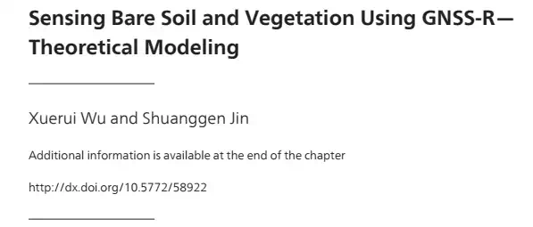
The tide gauge (TG) at the coast can measure relative sea level variations with respect to the coast (Woodworth and Player, 2003). We use the tide gauge (TG) data provided by the Permanent Service for Mean Sea Level (PSMSL). The PSMSL dataset consists of over 2100 tide gauge stations in the world, and the observation data are provided to a common benchmark-controlled datum (PSMSL, http://www.psmsl.org/). The time series of monthly TG averages from the revised local reference data are used to analyze the relative sea level changes. We selected 347 tide gauge data continuous observations from January 1993 to December 2012. Figure 1 shows the global distribution of tide gauge stations. Some TG data with missing over 4 consecutive months in one year are not excluded and other all available TG data are used.
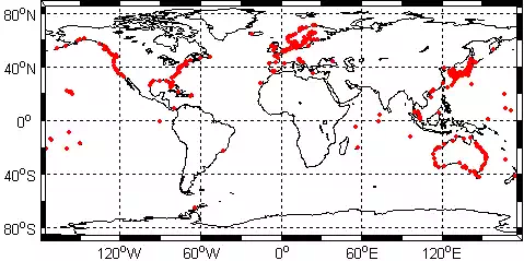
Since tide gauge measures the relative sea level changes along the coasts, so vertical land motion should be observed and added to get absolute sea level change. Now GPS could precisely monitor the land motions in an absolute reference frame [20, 21, 22]. Here we use global GPS time series provided at SOPAC (Scripps Orbit and Permanent Array Center) from January 1993 to December 2012, including 1459 consecutive observation stations (Figure 2). Details about the GPS data processing are available at the SOPAC website (http://sopac.ucsd.edu/processing/). In addition, the impact of the glacial isostatic adjustment (GIA) on the vertical ground motion is corrected [14, 27]. In this paper, for each TG station, we select co-located GPS station with latitude and longitude of less than 2 degrees. Then we regard the vertical crustal movement measured by the GPS as the crustal movement at TG stations. Some TG stations do not have the co-located GPS stations nearby. For these TG stations, we choose the all GPS stations within a perimeter of 10 degrees, and use a linear interpolation to obtain the vertical crustal movement at that point.
SATELLITE ALTIMETRY
The sea level changes along global coasts are studied using the global merged Sea Level Anomaly grid (SLA) data from Archiving, Validation and Interpretation of the Satellite Oceanographic data (AVISO) in France. More information can be found at www.aviso.altimetry.fr. The data set is a combined solution from the ERS-1/2, Topex/Poseidon (T/P), ENVISAT and Jason-1/2 altimetric satellites. The altimetric data set is 7-day time resolution at 0.25°×0.25° grids from January 1993 to December 2012 (AVISO, 1996), with respect to the CLS10 Mean Sea Surface. All related errors are corrected, such as tropospheric and ionospheric delays, solid Earth and ocean tides, pole tide, the Inverted Barometer (IB) response of the ocean and instrumental bias [10].
GRACE MASS AND STERIC COMPONENTS
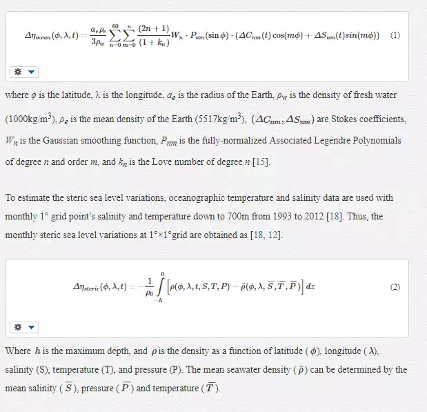
The global sea level changes from satellite altimetry include the steric and non-steric variations. To estimate the mass-induced sea level variations, the monthly GRACE solutions (Release-05) from the Center for Space Research (CSR) at the University of Texas, Austin are used from January 2003 to December 2012. Firstly, since the GRACE is not sensitive to C20, the C20 coefficients are replaced by Satellite Laser Ranging (SLR) solutions [6]. The coefficients of degree 1 are used from [33]. In addition, the 300km width of Gaussian filter and de-striping filter are used [12, 19, 34]. The postglacial rebound effects are removed using the GIA model of [27]. Furthermore, the land-ocean leakages are reduced as much as possible [36]. In order to obtain total mass variations, the GAD atmospheric and ocean model is added back [13, Willis et al., 2008]. Using the gravity coefficients anomalies the mass-induced sea level changes can be obtained [5, 24]:
Results and Discussions
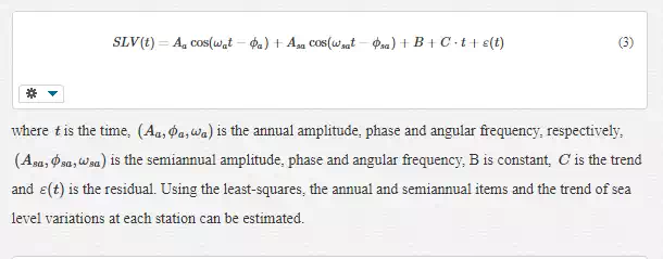
The total sea level change time series along the global coasts are obtained from Satellite Altimetry, Tide Gauge plus GPS, and GRACE Mass plus temperature/salinity-derived steric variations. For example, Fig.4 shows the sea level variation time series at the TG station ceu1with agreeing well each other. The sea level variation (SLV) time series have a strong annual and semiannual signals and the trend, which are expressed as [12]:

SECULAR SEA LEVEL CHANGES
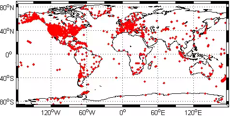
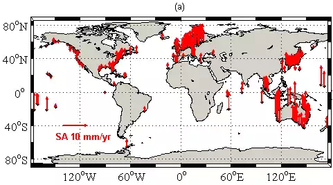
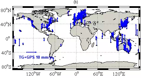
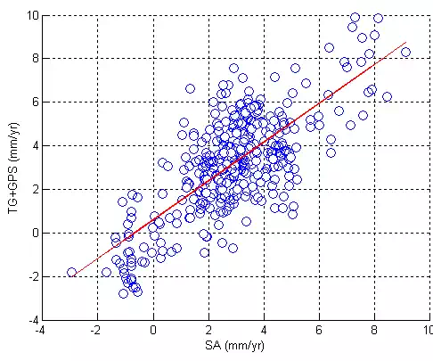
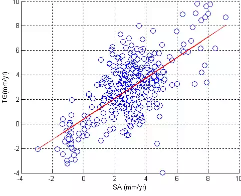
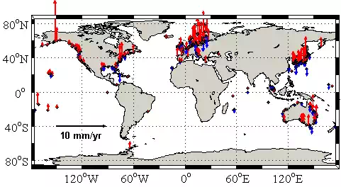
In this section, we focus on the trend of global coastal sea level changes. Figure 4 shows the long-term trend variations of the global 347 Tide Gauge stations from satellite altimetry (a), and Tide Gauge (b). Compared Fig. 5(a) with Fig. 5(b), it has clearly shown that at most TG stations, the satellite altimetry and TG+GPS results have a good agreement in secular trend. To further study the consistency between the two, we analyzed the correlation between each other shown in Figure 6. For the trend, the correlation coefficient between SA and TG+GPS time series is 0.75. We also calculated the correlation between SA and TG shown in Figure 7, and found that the correlation coefficient between SA and TG time series is 0.64. Compared Figure 5 and 6, we can find that when using GPS data for vertical crustal correction, the results of satellite altimetry and tide gauge stations have a better agreement, the correlation coefficient is increasing from 0.64 to 0.75. In order to study the influence of vertical crustal correction in each TG station, Figure 7 represents the difference between SA and TG+GPS trends at each TG station, where the red arrow indicates TG+GPS and SA results are closer, while the blue arrow indicates the result of TG and SA are closer, and here the length of the arrow represents the magnitude of the difference between each other. As can be seen from Figure 8, when using GPS data for vertical crustal correction, almost 75% TG stations’ results are much closer to the satellite altimetry results. In Figure 8, we can find that the 25% TG stations almost focus in the absence of co-located GPS stations (see Fig.3). It should be noted that the vertical crustal movement caused by many geophysical factors, including the main seasonal variations, as well as smaller magnitude (mm/yr) linear motion together with many large amplitude periodic motion, and vertical movement in different locations are different. Therefore, when use linear interpolation to determine the vertical displacement at the TG stations without co-located GPS stations, it will induce some errors.
SEASONAL VARIATIONS OF SEA LEVEL
Excluding the secular seal level change, the seasonal variation of sea level is significant. Since the sea level variations along global coasts are highly non-uniform, here we focused on analysis of the seasonal sea level changes with case study along the European coasts. We have selected 31 TG stations and used satellite altimetry, tide gauges, GPS, GRACE (satellite gravimetry) and Ishii oceanographic data to analyze and investigate the sea level variations along the European coasts. Since the semiannual amplitude is small when compared to the annual amplitude, the annual variations are main analyzed. Figure 9 shows the amplitudes and phases of annual sea level changes along the South-west European coasts at 31 TG Stations from Tide Gauge + GPS (blue), satellite altimetry (red line), and GRACE Mass + Steric sea level changes (green) from 1993 to 2012 (GRACE mass term is just from 2003 to 2012) [12]. Totally speaking, annual amplitude and phase of sea level variations along the European Coasts have a good agreement in three independent observations.

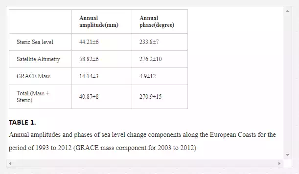
In order to further research the relationship in the three results from different techniques, we calculated the correlation coefficients between SA, TG+GPS and GRACE Mass+Steric. For the annual amplitude, the correlation between SA and GRACE Mass + Steric time series is 0.5, and the correlation between SLA and TG + GPS time series is 0.79. For the annual phase, the correlation between SA and GRACE Mass + Steric time series is 0.39, and the correlation between SA and TG + GPS time series is 0.80. The TG + GPS results agree better with altimetry results than the GRACE Mass + Steric results both in annual amplitude and phase. Furthermore, we find that the annual variations of sea level changes along the Southwest European coasts are mainly driven by the steric component (Table 1). The annual amplitude of steric sea level is 44.21±6 mm, while the mass-induced sea level amplitude is 14.14±3 mm, which is almost a quarter of steric component. For the annual phase, the maximum value of annual GRACE-derived mass sea level changes appears in January, almost six-seven months later than the steric sea level changes with the maximum value in August [12]. The annual phase differences of GRACE Mass + Steric results with respect to the TG + GPS and SA may be the different used geophysical models in GRACE, Satellite Altimetry and TG, which should be further investigated,
EFFECTS AND DISCUSSIONS
Totally speaking, the results have good agreements in annual variations and the trend between satellite altimetry, TG + GPS and GRACE Mass + Steric global coastal sea level variations from1993 to 2012, but there are still some differences. For GRACE results, GRACE instruments noises and measurement errors will affect our estimates; secondly, the atmosphere and ocean models are not accurate [16]; and the other one is due to the low spatial resolution and land-ocean linkage errors. For GPS results, lots of unknown errors are existed, such as mapping functions, the antenna phase center variations, bedrock thermal expansion and contraction, multipath effects and so on [17, 31].
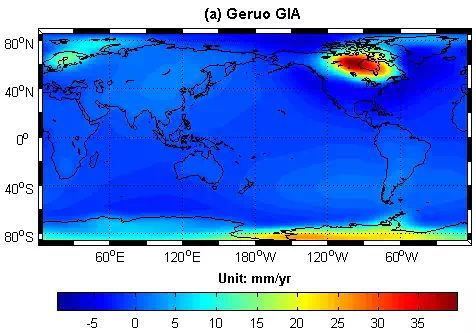
In addition, the GIA models are still uncertain in Southwest European coasts. When we use different GIA correction models, the results have some large differnces. Figure 10 shows the two different GIA models’ estimates in the global. At present, the commonly used GIA model is Peltier09 and Paulson07 GIA model (Geruo13 is a modified version of the Paulson07 model, and Peltier12 is a modified version of the Peliter09 model) [14, 30). Fig.10(a) is the result from Paulson’s GIA model depending on the ICE-5G model and VM2 mantle model [14, 27]; the Fig.10(b) is the estimate from Peltier’s GIA model, which depends on the ICE-5G v1.3 deglaciation model and VM2 mantle model with a 90 km lithosphere [28, 29, 30]. It can clearly be seen that the two models in North America, Canada and the northern part of the Antarctic region, the difference between the two GIA models is larger, and in the central and southern Asia, South America, the trend of Peltier12 model is obviously greater than Geruo13 GIA model. Therefore, the uncertainty of GIA models is one of error sources in the trend of sea level variations estimated by the GPS and Tide Gauges.
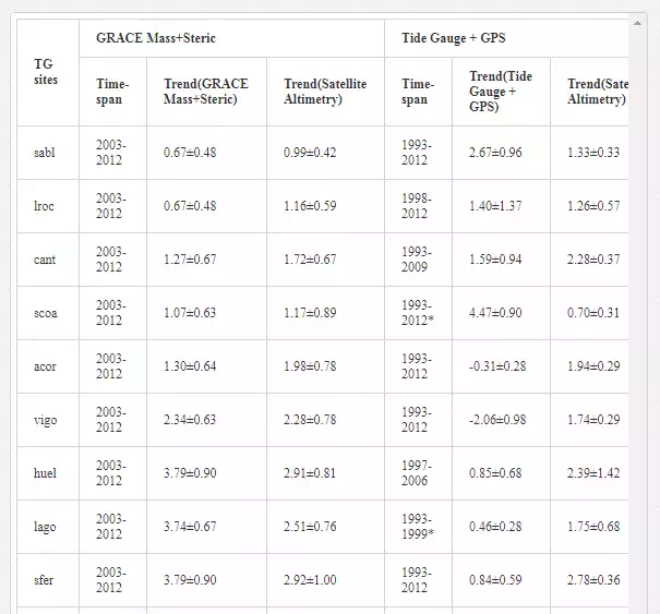
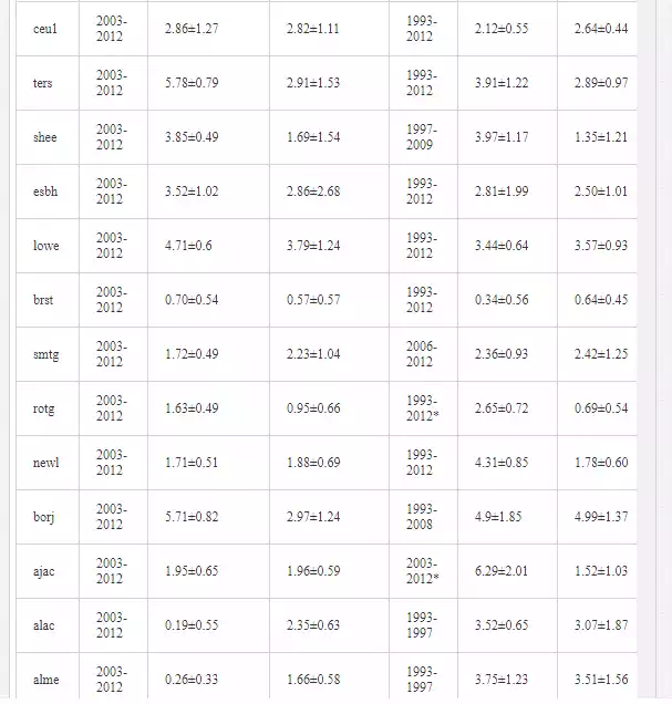
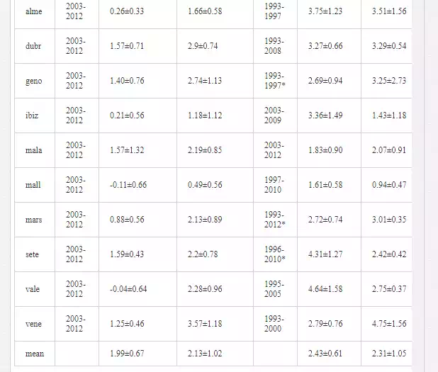
In addition, observation time of three kinds of independent techniques cannot be the same completely, which will also affect the results. In order to check the effect of observation time span on the trend, the trends are calculated from satellite altimetry, GRACE and TG for the same period of 2003-2012, respectively (Table 2). The correlation coefficient between SA and TG + GPS trends is improved from 0.51 to 0.61 and the correlation coefficient between SA and GRACE mass + steric trends is improved from 0.30 to 0.45.
Conclusion
In this chapter, the sea level variations along the global coasts are investigated in details from satellite altimetry, GPS, tide gauges, GRACE and Ishii oceanographic data, particularly in European coasts. For the secular trend, the results show that when using GPS data for vertical crustal correction, the results of satellite altimetry and tide gauge stations have a better agreement, and the correlation coefficient is increasing from 0.64 to 0.75. Furthermore, seasonal variations of sea level are further investigated with case study along the European coasts. The annual variations of sea level change along the European coasts from the TG + GPS are well consistent with satellite altimetry with correlation coefficient of 0.79 in annual amplitude and 0.80 annual phase at 31 co-located GPS and TG stations from 1993 to 2012. At most stations, the annual phases of the three techniques results also agree well. The annual amplitude of steric sea level variations is 44.21±6 mm, while the mass-induced sea level amplitude is 14.14±3 mm, which is almost a quarter of steric component. The annual variations of sea level changes along the European coasts are mainly driven by the steric contributions. Therefore, these results indicate that the co-located tide gauge and GPS well estimate the annual signals and the trend of sea level changes along the coast.
We are grateful to thank the Scripps Orbit and Permanent Array Center (SOPAC), the Permanent Service for Mean Sea Level (PSMSL) for providing GPS and Tide Gauge data and Center for Space Research (CSR) for providing the GRACE data. This research is supported by the Main Direction Project of Chinese Academy of Sciences (Grant No. KJCX2-EW-T03), National Natural Science Foundation of China (NSFC) Project (Grant No. 11173050) and Shanghai Science and Technology Commission Project (Grant No. 12DZ2273300).