High-order Ionospheric Effects on GPS Coordinate Time Series

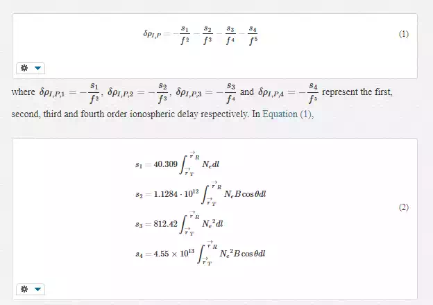
Weiping Jiang¹, Liansheng Deng² and Zhao Li³

^[1] Research Centre of GNSS, Wuhan University, Wuhan, China

^[2] School of Geodesy and Geomatics, Wuhan University, Wuhan, China

^[3] Faculté des Sciences, de la Technologie et de la Communication, University of Luxembourg,, Luxembourg

Introduction

Global positioning system (GPS) coordinate time series are used extensively for investigating various geodesy and geophysics problems [1,4,24], e.g., global and regional reference frame establishment, deformation monitoring for tectonic plate movement, etc. Until now, many investigators have studied the characteristics of GPS coordinate time series, and its general features are relatively well known, among which the seasonal signals, defined as annual plus semi-annual variations, are pervasive under the approximately power-law backgrounds [27,29,34,39,41]. Overall, the residual power declines with increasing frequency, and is consistent with a flicker noise distribution plus white noise at high frequencies. An in-depth understanding of the related mechanisms that cause seasonal variations is expected to separate signal from noise better in the GPS positions. Possible errors include both geophysical effects (e.g., mis-modelled tides and unmodelled non-tidal loading displacements) and technique-specific errors (e.g., long-term orbit mis-modelling and long-wavelength multipath effect). Previous researches find that geophysical models could only interpret ~40% of the seasonal power. Much of the residual seasonal power is most likely caused by unidentified GPS technique and/or analysis errors [6, 12].

Ionospheric delay is one of the main error sources in GPS positioning. At present, most GPS precise data processing only consider the first order ionospheric delay correction, which consists of more than 99.9% of the ionosphere effects and is usually removed by forming an “ionosphere-free” linear combination (LC). The remaining terms, that are the higher-order terms, however, do not cancel in the LC combination. The second order term is affected by both the ionospheric electron content and the geomagnetic field [31, 32], whereas the third order term is mainly affected by the ionospheric electron content and is much smaller in magnitude. At GPS frequencies, the fourth order and subsequent terms are negligible [32]. In recent years, higher-order ionospheric (HOI) effects, as one type of GPS technique-specific errors, have been studied on the GPS coordinates by many authors [3, 7,8,11,13,18,26]. Munekane analysed the influence of the second order ionospheric delay model [26]. Applied to regional and global networks, the model helped to furnish a quantitative explanation of the characteristics of the change of scale in the time series observed in the Japanese GPS Earth Observation Network (GEONET). Other authors have addressed the global GPS networks both with and without considerations of HOI effects. Comparisons of these solutions revealed systematic shifts in the site positions, reference frame origins, together with orbits and scale factors. They confirmed that ignoring HOI delay could lead to magnitude of centimeter-level or even larger error in positioning. It could also generate spurious diurnal, semi-annual and annual signals in the GPS coordinate time series, which might be wrongly interpreted as tidal effects or crustal movement.

To investigate the contribution of HOI terms, including the second and third order delay, to the GPS coordinate time series would do benefit to establish a more precise terrestrial reference frame and make a more reasonable interpretation of the motion characteristics of the tracking stations in the crustal monitoring network. Because of these reasons, the first and second GPS reprocessing campaign implemented by IGS analysis centre have already incorporated the second order ionospheric delay correction into the latest data processing strategy[1] - .

In this chapter, we focus on the effects of the second- and third-order ionospheric terms on the characteristics of GPS coordinate time series in terms of seasonal variations (the word “seasonal” mainly is used to represent both annual and semi-annual periods) and noise amplitudes, following the approach of previous authors concerned with coordinate-level effects [7, 8]. Although the effects of differential bending of the GPS signals due to the ionosphere propagation have been noted at the signal level, they are beyond the scope of this chapter. The ionospheric maximum years from 1999 to 2003 are selected for investigation. These years mark the peak of the previous solar cycle [16,25,28]. It permits a more complete understanding of the effects on coordinate time series and facilitates the analysis of recent GPS coordinate time series.

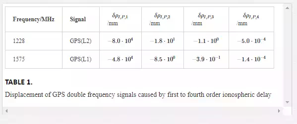
Firstly the modelling method of HOI correction in GPS precise data processing is investigated, and then the impact of ionopsheric delay with different orders on the GPS dual-frequency carrier signals is quantified. Based on this, the GPS data of 104 evenly distributed IGS sites are reprocessed using GAMIT. Analysis is begun by comparing the differences caused by HOI effects in terms of differences in site coordinates and velocities. Then the periodic characteristics and noise amplitudes of coordinate time series with and without HOI corrections are assessed. The evaluation of the solutions is based on the comparison of the coordinate time series characteristics of each coordinate component.

HOI delay model

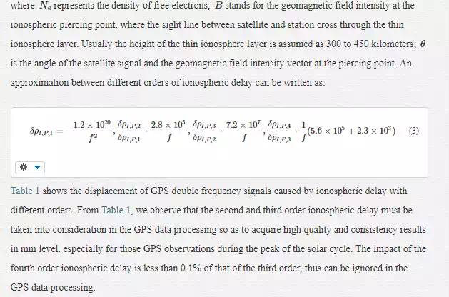
The ionospheric delay on the carrier phase that extended to the fourth order can be written as [30]:

GPS data processing

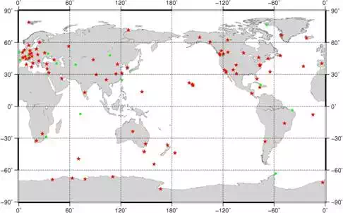
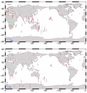
The IERS convention 2010 recommends that the impact of HOI delay must be taken into consideration when establishing future terrestrial reference frame [30]. In order to determine the impact of HOI delay on the coordinate time series of IGS sites, a contrast experiment is set up based on the latest model recommended by IERS convention 2010 and recent published results to reprocess the GPS data of 104 evenly distributed IGS sites. In experiment A, only the first order ionospheric delay is calculated, while in experiment B, the impacts of the second and third order ionospheric delay are considered. Except for the different way in dealing with the ionospheric delay, all the other strategies are exactly the same in both runs. Figure 1 shows the spatial distribution of the IGS stations. Stations are selected from part of the ITRF sites with high geodetic quality, which satisfy the following criteria: (a) evenly distributed worldwide; (b) continuously observed for at least 3 years; (c) locations far from plate boundaries and deforming zones; (d) velocity accuracy better than 3 mm/yr. During the calculation, we use the GAMIT/GLOBK (V10.4) as our platform [9, 10].

Users could realize HOI delay correction in GAMIT 10.4 by setting the parameters Ion model as GMAP and the Mag field as IGRF11 or DIPOLE in the control file called sestbl. At the same time, a new folder called ionex should be created under the project directory to save daily ionosphere file. After that, we have to switch on the -ion command when using sh_gamit to process the data, since the default setting is only calculate the first order ionospheric delay.

The global Vertical Total Electron Content (VTEC) data read by GAMIT are provided by the Center for Orbit Determination in Europe (CODE)[2] - [9, 14], with a temporal resolution as 24 hours before day 87, 1998 and 2 hours after that. Based on both the temporal resolution of the VTEC product and the strong ionosphreic activity, we choose the time span from year 1999 to 2003. Besides, considering the superiority of the International Geomagnetic Reference Field (IGRF) to the co-axial tilting dipole magnetic field model [31], we choose the latest IGRF11 to acquire the geomagnetic field intensity 

BB

 at the ionospheric piercing point, which is needed to calculate the second order ionospheric delay. The height of the ionosphere layer is assumed as 450 kilometers from day 87, 1998 [9]. Moreover, since the IGS stations move slowly within one week, and can be ignored, we only process the GPS data on every Wednesday, which could not only show the long term trend of IGS stations, but could also improve our working efficiency.

In our data processing, several parameters are resolved simultaneously, including site coordinates, earth orientation parameters, satellite orbits, tropospheric delay and the horizontal gradient parameters [17]. The stations are given loose constraints, among which the constraints of 5cm are set to IGS core stations, and 1dm to the non-core stations [22]. Ten degree is chosen for the satellite cut-off elevation angle, and the observations are weighted with site-specific, elevation-dependent weighting based on an assessment of the post phase residuals [15, 22, 38]. Corrections have been implemented for solid earth tide, ocean tide and pole tide, among which the FES2004 model is used to calculate site displacement due to ocean tidal loading [23]. Absolute antenna phase center offsets and variations are used [35]. Vienna Mapping Function 1 (VMF1) troposphere mapping functions are used to calculate the tropospheric delay [5]. Atmospheric tidal correction and non-tidal loading corrections are not applied [22, 30]. Pressure and temperature for the a priori zenith hydrostatic delay are provided with receiver-independent exchange (RINEX) meteorological files (.m) and values from VMF1 [37]. After obtaining the weekly baseline resolutions, datum transformation is performed with GLOBK to obtain sites’ coordinate time series and velocities under the ITRF [36].

Coordinate time series analysis methods

SPECTRAL ANALYSIS METHOD

Spectral analysis can be used to investigate the frequency characteristics of coordinate time series, including the main cycle components and the periodic variations. The Lomb-Scargle periodogram method is used in this chapter. This method overcomes the shortcomings of the classical periodogram, which can only be applied to equidistant data and to search for cycles in equidistant data, and is widely used in computing the noise spectrum of GPS coordinate time series [24, 41, 44]. The basic idea of this method is to obtain an improved periodogram through the redefinition of every angular frequency by introducing a time lag ττ

MAXIMUM LIKELIHOOD ESTIMATION METHOD (MLE)

The GPS site velocity error tends to be overestimated approximately 4 times or even by an order of magnitude if the effect of coloured noise is ignored, thus producing incorrect geophysical interpretations [24,39,19-21]. To incorporate the effect of coloured noise, the best approach is to apply MLE to estimate the modelling parameters and the noise components simultaneously.

Considering the influence of the colored noise, daily solution observation sequence of each coordinate component can be modeled as follows [27]:

Data analysis and discussion

In this section, the impact of HOI delay on the variations of stations’ coordinates, velocities, and the variations of the GPS coordinate time series are investigated.

EFFECTS ON COORDINATES

To investigate HOI effects on site coordinates, the solutions from experiment A and experiment B are compared. Considering the reliability of the limitation of the observation processing span, only sites with continuous time series having a length of more than 2.5 years are included. For sites interrupted by antenna change or earthquakes or other causes, the data span having the longest time interval for the same station is used. Figure 2 shows the global site coordinate differences resulting from the modelling of the HOI corrections. The values shown in this figure are the differences in the final coordinates that are estimated from the weekly baseline solutions using the Kalman filtering method applied in GLOBK software. A pattern of high-latitude sites shifted northwards and equatorial sites shifted southwards is observed in the horizontal components, and the former sites have smaller offsets than the latter sites, as also found by reference [31] and reference [8].

EFFECTS ON VELOCITIES

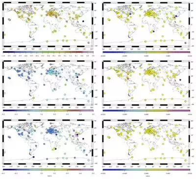
Figure 3 shows the spatial distribution of stations’ velocity and its uncertainty difference in the North, East and Up component between experiment A and B. From Figure 3, we observe that HOI delay has some impact on the long term velocity of IGS sites, but has almost no impact on its velocity uncertainty. The mid-to-low latitude stations are most affected, while those in the high-latitude region suffered small effects (except for OHIG). With respect to the Up component, the maximum velocity difference reaches up to 1mm/year for stations near the equator, e.g. GUAM in the West Pacific and KOKB in Hawaii. Compared with the Up component, the horizontal components are relatively less affected with maximum velocity difference of no more than 0.5mm/year, and can be neglected. Another interesting phenomenon is that ignoring HOI delay may lead to over-estimation of the Up component for stations in the southern hemisphere and at the same time under-estimation of stations’ vertical velocity in the northern hemisphere. Therefore, HOI delay must be considered in the high precision data processing for equatorial stations, so as to acquire more reliable vertical velocity in the application of meteorology and geodynamic studies, such as postal glacial rebound, sea level change, etc.

IMPACT ON THE SCATTER OF THE GPS COORDINATE TIME SERIES

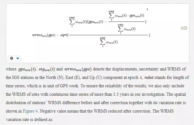
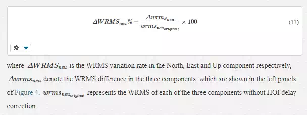
To investigate the impact of HOI delay on the scatter of stations’ displacement time series, the WRMS of coordinate time series of IGS sites both before and after HOI delay corrections are separately calculated. Let 

ωneu(i)=1/signeu(i)2ωneu(i)=1/signeu(i)2

, the WRMS of GPS coordinate time series can be calculated by:

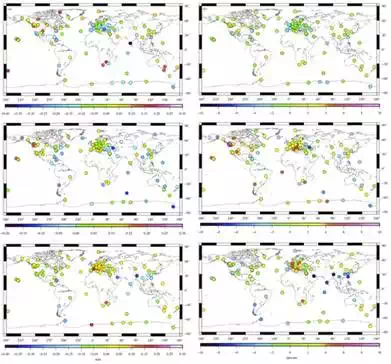
From Figure 4 we can see that, most stations’ vertical WRMS decrease after HOI delay correction, accounting for 66% of the total stations. The biggest improvement gathers near the equator, for example, the HOI delay could explain 4% of the vertical WRMS at station IISC (13°N). The WRMS variation in the North component shows remarkable regional characteristics. 47% of the stations’ WRMS decreased, and most of them gathered in South Asia, with WRMS reduction between 4% to 10%, including 5 stations in China, among which the WRMS reduced by 10% for station LHAS.. Different from the Up and North components, the East component does not yield big improvement after higher order ionospheric delay correction, among which only 33% of the stations’ WRMS reduced, and most of them located in the Oceania, America and coastal areas around Asia. Besides, we also notice that the WRMS in the North component of most stations in Europe are increased by 5% to 10% after HOI delay correction. Further work is still required to determine the reason.

EFFECT ON THE SPECTRUM CHARACTERISTICS OF THE GPS COORDINATE TIME SERIES

To study the periodic variations caused by HOI corrections, detailed study of the periodic characteristics and differences between solutions is restricted to only those sites with more than 4 years of data (not necessarily consecutive), without known offsets caused by hardware changes and without known coseismic and/or postseismic deformation signals or identifiable effects of snow covering the antenna. The selected sites are shown as red stars in Figure 1. The Lomb-Scargle periodogram method is applied to calculate the power spectral density (PSD) of the coordinate time series using CATS [42]. After obtaining the spectra files, the periodic spectra diagrams are plotted for the N, E and U components.

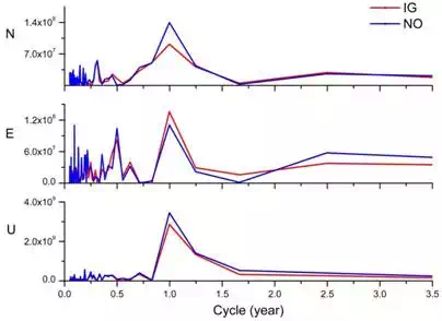
Figure 5 shows the spectra diagrams for the IISC site. Red lines represent the post-correction (IG) results and blue lines represent the pre-correction (NO) results. In this figure, periodic signals over 3.5 years are truncated to show the short-period signals clearly. For both two runs (IG and NO), there are periodic characteristics shown in the GPS coordinate time series. However, the corresponding main power spectra values are changed with different directions. The U component show a more obvious periodic characteristic than the N and E components, as its power value is approximately 5-10 times greater than those of the other two components. Additionally, signals with small periodicity (less than 0.5 year) are found in all components. In general, the main contributors to seasonal variations include gravitational excitation, thermal origin and hydrological dynamics [6, 33]. Ocean tides, solid Earth tides and atmospheric tides, which are associated with gravitational excitation, have been modified in the GPS carrier phase data processing using relatively precise theoretical models. Thus, effects of the thermal origin and hydrological dynamics may produce variations in our GPS coordinate time series. Additionally, the thermal noise of the antenna, local multipath effects and model errors such as satellite orbital models, tropospheric delay models and other technique-specific system errors can induce seasonal deformation at the sites [2,12,22,35,42].

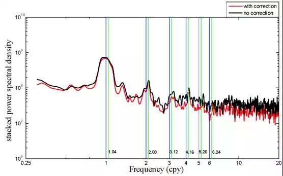
To display the overall variations caused by HOI corrections clearly, we stack all the spectra of the selected sites for two runs by component and smoothed with a Gaussian smoother. Figure 6 shows the analysis results. Vertical dashed lines are plotted in Figure 6 to indicate harmonics of 1.0 cycle per year (cpy). We can see that no matter with or without HOI corrections, all the three components exhibit very similar behaviour, except that the E component without HOI corrections shows a different pattern. Peaks are evident at harmonics of approximately 1 cpy up to at least 6 cpy. Although the two lower frequencies appear to match the annual and semi-annual periods, it becomes progressively more apparent at the higher frequencies that harmonics of 1.0 cpy do not fit the observed peaks well. It is also evident that the power remains on the high-frequency sides of 1.0 and 2.0 cpy. Vertical dashed lines are also drawn for the harmonics of 1.04 cpy, and they fit the observed sub-seasonal spectral peaks well, especially for the relatively narrow 3rd, 4th, 5th and 6th peaks of all three components. This is a strong indication that the observed seasonal bands actually consist of 1.0 cpy, 2.0 cpy together with 1.04 cpy, which is called the GPS “draconitic” year [34]. In addition to the 1.0 cpy and 2.0 cpy harmonics (annual and semi-annual harmonics), the indications of 1.04 cpy harmonics also persist largely unchanged after HOI corrections, especially for the U component. Moreover, they are even more remarkable after corrections, especially for the 4th, 5th and 6th peaks in the N and E components. Therefore, HOI corrections may not be the main contributions to our inferred harmonic generating tone at 1.04 cpy. Ignoring these corrections can even submerge this type of harmonic.

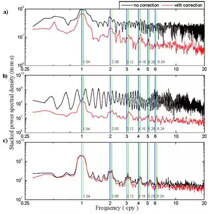
Before corrections, the stacked results for the E component do not show a regular pattern (obvious peaks for the annual and semi-annual signals), which is unlike the other two components. After corrections, more consistent and normal variations are shown in the E component, which is also true for the high-frequency harmonics of N component. If we ignore these corrections, the result can be a spurious signal, and cause an unreasonable seasonal pattern for the E component. After HOI corrections, there are overall decreases for all seasonal amplitudes (such as annual, semi-annual, 1.04 cpy), especially for the N and E components, indicating that these corrections can weaken the noise existing in the global coordinate time series. We will examine this question more closely in the next section.

NOISE ANALYSIS

In this section, the Maximum Likelihood Estimation method (MLE) is applied to analyse the noise characteristics of the coordinate time series. In the beginning, the optimal noise model is determined. Under the optimal noise model, the effects of HOI corrections on the site noise amplitudes and seasonal signals are assessed.

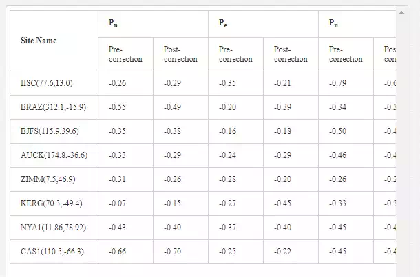
The spectral index of the coordinate time series is first calculated to help determine the potential noise type. Table 2 lists the spectral index of the selected sites located in different latitudes. Here sites are selected mainly considering that they are located in low-, mid- and high-latitude areas from two hemispheres. As shown in Table 2, the noise spectral index values for the three components at all tabulated sites are between -1 and 0 whether HOI effects are considered or not. The same result holds for the other sites except that the values for a few sites range between -1 and -2. The coloured noise still exists in the coordinate time series. Therefore, it can be inferred that coloured noise is present at all the selected sites, and that HOI corrections cannot remove this kind of coloured noise.

Based on the above results and previous studies involved in noise analysis, four types of noise model are selected here to determine the optimal noise model for the global sites. The selected noise models are white noise (WN), flicker noise (FN), random walk noise (RW) and power law noise (PL). In general, the larger the MLE value, the more effective the noise model is [24, 19-21]. According to the Langbein experiment, using a significance level of 95%, we can distinguish two different noise models if the difference between the MLE values of the two models is greater than 3.0. In this chapter, the white noise model (WN) is used as the null hypothesis. We compare the other three combined models (white noise plus flicker noise (WN+FN), white noise plus random walk noise (WN+RW), and white noise plus power law noise (WN+PL)) with this hypothesis model.

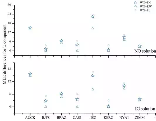
The MLE differences for different models relative to WN are shown in Figure 8 for the selected sites. Y-axis represents the difference values. The site names are shown on the x-axis. Here only the U component results are shown (similar results can also be found for N and E components). The MLE differences can be found to distinguish between different noise models. Overall, compared with the WN model, both the MLE differences for WN+FN and WN+PL are greater than 3.0, and the differences can be distinguished easily. The RW+WN noise model is not as obviously different from the WN model, and the RW noise does not make a marked difference. After HOI corrections, the MLE differences for most sites remain unchanged. According to the noise model determination method defined above, HOI corrections have little influence on the determination of the optimal noise model for global sites. Therefore, the same optimal noise model can be selected for both runs. Given the small MLE differences between WN+FN and WN+PL and the uncertainty of the WN+PL model in determining the noise components and other parameters, the WN+FN model is selected as the optimal noise model. In the following analysis, all the results are obtained under this optimal noise model.

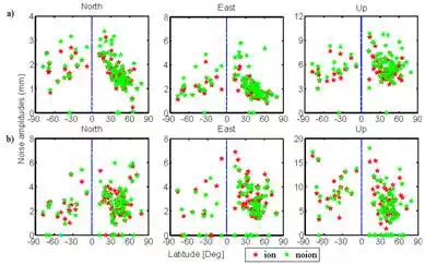
We estimate the noise amplitudes for each coordinate component of the stations for both runs. Figure 9shows the amplitudes of white noise and flicker noise. We split them in Figure 9 to denote the noise amplitudes variations of each noise type as a function of latitude. Zero value in Figure 9 means that the maximum likelihood estimation algorithm fails to distinguish the white or flicker noise coefficients. Table 3 lists the average noise amplitudes of sites located in different latitudes.

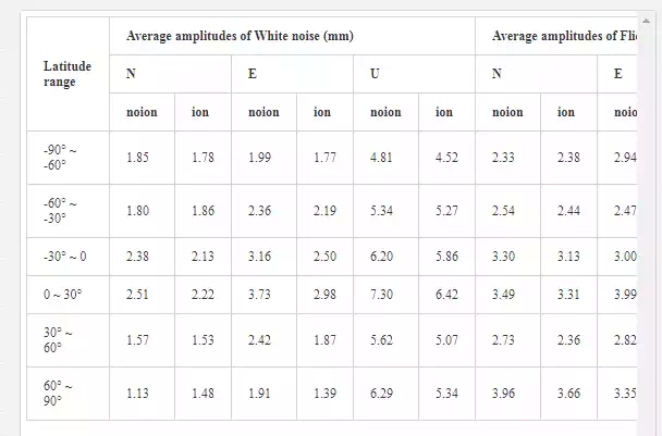
Generally speaking, variations of the amplitudes of white noise and flicker noise are latitude dependent. The noise amplitudes decrease as the latitude increases. The WN variations are more obvious than FN. This relationship has also been found in reference [24] and [41]. After HOI corrections were applied, there is an overall decrease in noise amplitudes, whereas the dependence of the variation in noise amplitudes on latitude still remained. Although HOI corrections can produce regional shifts at given sites and larger coordinate differences on mid- and low-latitude areas (Figure 2), the principal source of latitude-related variations in noise amplitudes may not be related to these corrections. It is worth noting that the corrections as modelled are not perfect, so there could be errors in the model. For most sites, the flicker noise amplitude is greater than that of the white noise, especially in the U component. Different noise amplitudes are found in different components for the same site. For both white noise and flicker noise, the noise amplitudes of the N and E component are smaller, and the noise amplitudes of the U component are the greatest. This is consistent with the lower precision of the U component relative to the N and E components. From the above results, we conclude that HOI corrections may not improve the precision of the U component substantially.

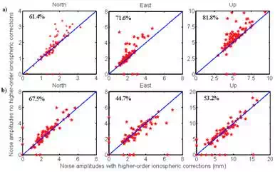
Figure 10 further shows the variations in noise amplitudes after HOI corrections. We added “x=y” diagonal line in figure to see deviations more clearly. The farther the points locate to the diagonal line, the greater the amplitudes changes are. The percentage of stations whose noise amplitudes are reduced by the HOI corrections is labelled on the plot. A comparison of the solutions from IG and NO shows that amplitudes of both WN and FN generally decrease for most sites, and the WN amplitudes decrease more remarkably after HOI corrections. For flicker noise, the amplitudes of 67.5% of the selected sites exhibit a decrease in the N component and yield the most satisfactory results. Compared with flicker noise, white noise yields a more satisfactory result for the global sites in terms of the percentage of sites with decreasing amplitudes (61.4%, 71.6% and 81.8% for N, E and U, respectively). Based on our results, HOI effects can maximallyexplain 44.02% (NICO), 91.10% (NOT1) and 49.8% (NICO) of the WN amplitude in the N, E and U components, respectively. The NICO and NOT1 sites are both located in mid-latitude areas (35°~37°N). For FN, the noise amplitudes decreased most at the same site, ANKR (39.88°N), and the summed proportions were 67.63%, 53.59% and 71.30% for the N, E and U components, respectively. For the global sites, the total noise amplitudes decreased, and HOI corrections must be considered if GPS coordinate time series are used to interpret geophysical phenomena. Moreover, noise amplitude variations caused by HOI corrections differ for sites in different areas, and the amplitudes of the sites in mid- or low- latitude regions show greater variations than those in other areas. Therefore, separate analysis and comparisons for different areas are recommended to obtain more meaningful conclusions.

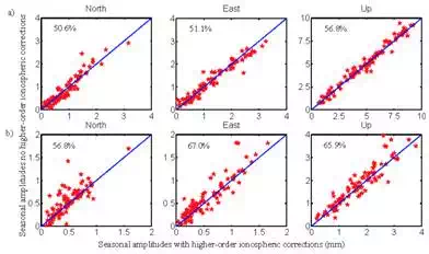
SEASONAL AMPLITUDE VARIATIONS

Section 5.4 shows that HOI corrections can weaken the overall amplitudes of seasonal signals qualitatively. Here, we quantify the effects of these corrections on seasonal signals. To have a clear understanding of seasonal signals variations at the global sites caused by HOI corrections, the annual and semi-annual amplitudes are estimated under the relatively optimal noise type (WN+FN) using MLE. The 1.04 cpy harmonics is not estimated considering that these anomalous seasonal signals lead to the errors of annual amplitudes’ great increase. Figure 11 shows the annual and semi-annual amplitudes estimated in the GPS coordinate time series both with and without HOI corrections. We also added “x=y” diagonal line in this figure as Figure 10. In general, the annual amplitudes decreased in height, but this trend cannot be generalised. For certain stations, the annual amplitudes even increased. HOI corrections are effective for approximately one-half of the GPS sites in the horizontal components. Also note that the semi-annual amplitudes of the sites are much more strongly affected by the corrections. It is probable that there is a good match between the seasonal amplitudes and the HOI corrections or that the observed variations are related to HOI effects. This finding is especially important to ensure a reliable interpretation of the non-linear variations in the station position time series. However, these results (Figure 11), as well as the noise amplitudes variations in Figure 9-10, show that HOI effects explain the data from the studied sites partially, especially in the height component, in terms of seasonal amplitudes’ variations for the global sites. The discrepancy could be due to loading model deficiencies or other systematic errors involving particular techniques, such as the thermal expansion and troposphere models.

Conclusions

In this chapter, the modelling method of the HOI delay correction is analysed and the magnitude of ionospheric delay with different orders on the GPS dual frequency carrier phase signals is determined. By reprocessing GPS data of evenly distributed IGS sites, the contribution of HOI delay to the global GPS coordinate time series is investigated. Our results indicate an overall improvement based on an analysis of the global sites. The following conclusions have been drawn:

HOI corrections can lead to big velocity variations of global IGS stations, among which the vertical velocity reaches up to 1mm/year for stations near the equator. Ignoring HOI delay correction will lead to over-estimation in the Up component of sites in the southern hemisphere and under-estimation also in the Up component of sites in the northern hemisphere.

The WRMS of coordinate time series in the Up component of stations near the equator and in the North component of stations in South Asia can be remarkably reduced if HOI delay correction is considered. Station LHAS in China exhibits the biggest improvement, and the WRMS in the North component reduced by 10%.

Whether or not HOI corrections are considered, the noise spectral index always ranges between -1 and 0, and HOI corrections have a negligible influence on the determination of the optimal noise model for our selected four noise types. In terms of noise amplitudes, although HOI corrections can produce regional coordinate shifts at given sites, noise amplitude variations related to latitude are still present. The principal source of the latitude-related variations in noise amplitudes may not be related to these corrections, and that HOI corrections may not substantially improve the precision of the U component. At most sites, the amplitudes of both white noise and flicker noise decrease as a result of the corrections, while the white noise amplitude showing a more remarkable change. The U component of the white noise amplitude decrease at 81.8% of all the selected sites as a result of the corrections, and the N component of the flicker noise amplitude decrease at 67.5% of all the selected sites. To obtain more meaningful conclusions, a separate analysis and comparison for different areas is still recommended.

The results of an analysis of stacked periodograms show that a common fundamental of 1.04 cpy, together with the expected annual and semi-annual signals, satisfactorily explaines all the observed peaks. HOI corrections may not represent the primary contribution to our inferred harmonic generating tone at 1.04 cpy. Nonetheless, there is a good match between the seasonal amplitudes and the HOI corrections, and the observed variation in the coordinate time series is related to HOI effects. HOI delays partially explain the seasonal amplitudes in the coordinate time series, especially for the U component. The annual amplitudes for all components are decreased for over one-half of the selected IGS sites. Additionally, the semi-annual amplitudes for the sites are much more strongly affected by the corrections.

The effects of HOI corrections on GPS coordinate time series further show that the application of HOI corrections should become a standard part for precise GPS data analysis. It is worth noting that more accurate correction models still need to be investigated. When contemplating routine inclusion of the higher-order corrections, one should consider generalizing these corrections by using a more accurate model of the Earth’ magnetic field and by using a more representative ionosphere which takes into account the ray-bending errors and the actual vertical spread of ionospheric density with altitude.

Acknowledgements

We thank Petrie, E. J, R. W. King and J. Ray for their constructive advices in the analysis. We also thank IGS for providing the GPS data and MIT for providing the GAMIT/GLOBK software. This research is supported by the Changjiang Scholar Program, the National Natural Science Foundation of China (41374033 and 41304007) and the National 863 program of China (2012AA12A209).

Notes

[1] - http://acc.igs.org/reprocess2.html

[2] - ftp://cddis.gsfc.nasa.gov/pub/gps/products/ionex/yyyy/ddd/codgddd0.yyi.Z