GPS-based Non-Gravitational Accelerations and Accelerometer Calibration
Andres Calabia1, 2 and Shuanggen Jin1
[1] Shanghai Astronomcial Observatory, Chinese Academy of Sciences, Shanghai, China
[2] University of Chinese Academy of Sciences, Beijing, China
Introduction
Within the process of deriving satellite accelerations from GPS observations, the reduced-dynamic Precise Orbit Determination (POD) approach is one of the most complete and accurate strategies. On the one hand, high-precision GPS solutions are independent of the user’s satellite dynamics but their solutions are more sensitive to geometrical GPS factors ([1] and [2]). On the other hand, a dynamical method estimates the satellite position and velocity at a single epoch for which the resulting model trajectory best fits the tracking observables. These dynamics involve the double integration and linearization of the Newton-Euler’s equation of motion, the force model, the parameters to be estimated and the orbital arc length. The combination of GPS observables with the dynamic approach can counterbalance the disadvantages of the dynamic miss-modeling and the GPS measurement noises (e.g., [3]) with the high GPS precision, the robustness of the dynamic approach and the use of additional force measurements and models (e.g., accelerometer measurements, time-varying gravity, irradiative accelerations, atmospheric drag, thruster firings, magnetic field, etc.). Since the POD products do not use to give information about the acceleration of the user’s satellite, accurate interpolation and subsequent numerical differentiation must be performed to the POD solution. For this purpose, a feasible methodology with the use of the arc-to-chord threshold is performed in this scheme of deriving satellite accelerations.
Non-gravitational accelerations are obtained by measuring the force to keep a proof mass exactly at the spacecraft’s center of mass, where the gravity is exactly compensated by the centrifugal force. Plus and minus drive voltages are applied to electrodes with respect to opposite sides of the proof mass, whose electrical potential is maintained at a dc biasing voltage. Unfortunately, this dc level is the source of bias and bias fluctuations of the most electrostatic space accelerometers. The non-gravitational forces acting on LEO satellites comprise the atmospheric drag, irradiative accelerations, thruster firings, the relative proof mass offset and the Lorentz force.
Several methodologies have been developed and applied for comparing the computed non-conservative accelerations with the accelerometer measurements. The non-conservative force models augmented with estimated empirical accelerations, for instance, have shown a good agreement with the accelerometer data [4] and were replaced with the accelerometer measurements in the reduced-dynamic POD, using a method with strong constraints in the cross-track and radial directions [5]. In [6], the non-gravitational accelerations were calculated as piece-wise constant empirical accelerations via the reduced-dynamic POD approach with a standard Bayesian weighted least-squares estimator. Here, the regularization was applied to stabilize an ill-posed solution and only the longer wavelengths were recovered, at best in the along-track direction, with a bias in the cross-track direction. It was concluded that no meaningful solution could be obtained in the radial direction.
Concerning the acceleration approach, where accelerations are derived from a numerical differentiation along precise orbits, the second derivative of the Gregory–Newton interpolation scheme was used in [7], a 16-order polynomial in [8], and a 6-order-9-point-scheme in [9]. After accelerations are calculated, the least-squares fitting can be applied, and the possible correlations between calibration parameters removed by using the (fitted) autoregressive-moving-average (ARMA) models [9].
However, results of the above mentioned studies were limited not only by the bias caused by applying a numerical differentiation, but also by the consequences of applying the least-squares estimation techniques. For example, the need of setting strong constraints or regularizations was probably caused by correlations from systematic errors. For this purpose, a new approach to accurately determine the GPS-based accelerations of GRACE mission was developed and applied in [10]. Along with the benefit of using high accuracy and precise methodology and models, these systematic errors were modeled and removed from the computed non-gravitational accelerations of GRACE. In the following sections, this new approach is reviewed in detail and the calibration of GRACE accelerometers is given as an example of its application for LEO satellite measurements.
Methods and models
ACCELERATIONS FROM GPS-BASED PRECISE ORBIT DETERMINATION
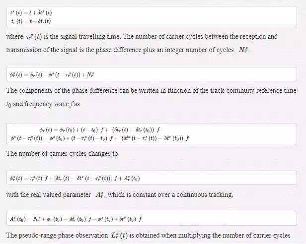
First, a brief description of the GPS-based POD strategy is given to understand what kind of solutions is dealt with. Both GPS satellite (superscript s) and GPS receiver (subscript r) experience a clock offset (δt), causing their respective internal time delays in the overall GPS system time t as:
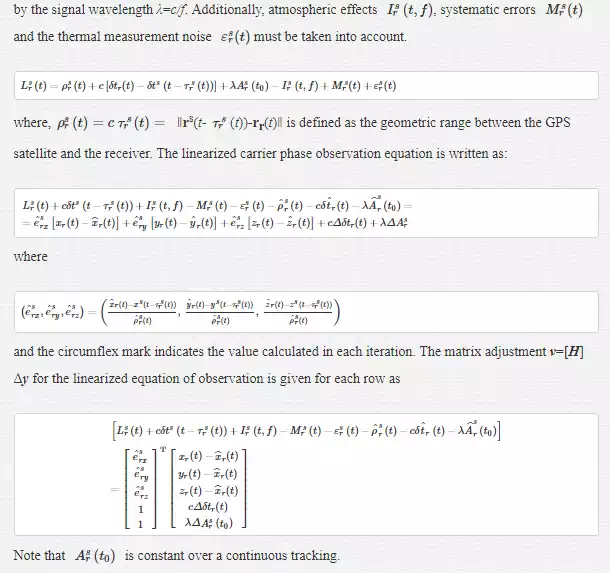
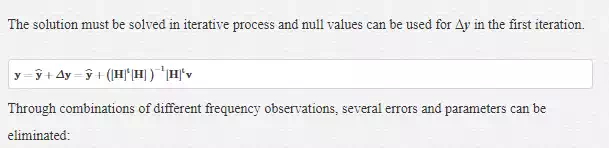
Through combinations of different frequency observations, several errors and parameters can be eliminated:
· Ionosphere free linear combination.
· Geometry-free carrier phase linear combination (to detect cycle slips).
· Wide-lane and narrow-lane linear combinations (for ambiguity resolution applications).
· Multipath combinations.
Detailed methodology can be found, e.g., in [11] or [12]. Differenced GPS observations has the advantage of eliminating or reducing several common error sources, such GPS satellite clock offsets and common biases from hardware delays. Distinguished by the carrier phase differencing level, high precision data processing procedures are basically:
· The zero-differences or Precise Point Positioning (PPP) processing, where un-differenced observations from a single GPS receiver are supplemented by pre-computed IGS ephemeris and clock products (e.g., [12, 11]).
· The single-differences processing, where the use of two receivers results in the cancelation of the satellite clock bias and common systematic errors Msr(t) Mrs(t).
· The double-differences processing, with the elimination of the receiver clock biases (e.g., [13, 14] and [15, 16, 17]).
· The triple-differences processing, which eliminates the time-independent errors ([18, 19, 20]).
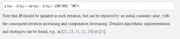
Detailed developments and algorithmic implementation can be found, e.g., in [21]. Regarding now the satellite dynamics, the first-order time-differential equations are
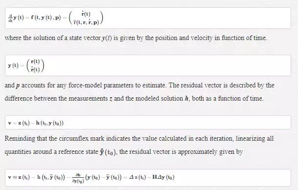
H gives the partial derivatives of the modeled observations with respect to the state vector at the reference epoch t0. The orbit determination problem is now reduced to the linear least-squares problem of finding Δy(t0). In first iteration, null values can be used, and the system solution is the correction to these values.
Since the POD products do not use to give information about the satellite’s acceleration, interpolation and subsequent numerical differentiation must be performed to the POD solution. In order to keep the error of interpolation small enough, a low-degree polynomial is not sufficient, high-degree polynomials introduce undesired oscillations, and the FFT approach is not considered in presence of data gaps and outliers [26]. The best alternative, as seen in [7], is to use a piece-wise interpolation, such as splines or Hermite polynomials. Different algorithms for interpolation were compared in [10], interpolating odd from even original samples, and the committed error evaluated by a simple difference between interpolated and original data. Finally, 8-data point piece-wise Lagrange interpolation was chosen, which provided a white noise error of standard deviation of ~10nm/s, from evaluating the error committed at 10 s sampling (odd from even original samples). Similar results were obtained when the piece-wise cubic Hermite interpolation was tested.
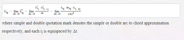
When calculating total accelerations by simple differentiation of velocities, the approximations to numerical derivatives have been found to produce large bias [9]. To avoid this error of arc-to-chord approximation [10], interpolated velocities must be differentiated by an increment of time (Δt), which minimizes the error committed at a given threshold. The modified three-point formula upgraded with the arc-to-chord threshold (Δt) is given by [10] in the form
TIME-VARYING GRAVITY FIELD EFFECTS
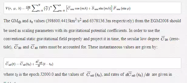
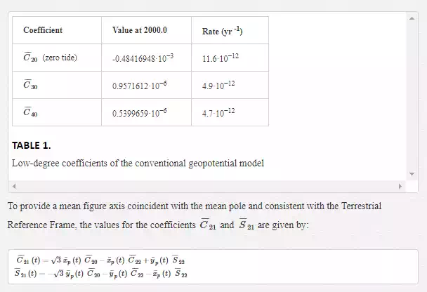
The conventional gravity model based on the EGM2008 [27], describes with Stokes’ coefficients the static part of the gravitational field and the underlying background for the secular variations of some coefficients. In addition, when computing the gravitational forces acting on the satellite, other time-varying effects must be taken into account. These include the third body tide caused by the Moon and Sun, the solid Earth tides, the ocean tides, the solid Earth pole tide, the ocean pole tide and the relativistic terms.
The geopotential field V at the point (r, φ, λ) is expanded in spherical harmonics with up to degree N as:
The gravitational acceleration of a third body on the satellite [22] can be described as a difference between the accelerations of the satellite and the Earth caused by a third body B

where rsat and rB are the geocentric coordinates of the satellite and of a third body of mass MB,respectively. Since accelerations on near-Earth satellites from other planets actions are relatively small (< 0.1nm/s2), only Luni-solar accelerations are calculated. Moon and Soon coordinates can be interpolated from the solar and planetary ephemerides (DE-421) provided by the Jet Propulsion Laboratory (JPL) in the form of Chebyshev approximations. The evaluation of these polynomials yields Cartesian coordinates in the ICRS for the Earth-Moon barycenter b⨁⊘ and the Sun b⊙ with respect to the barycenter of the solar system, while Moon positions r⊘ are given with respect to the center of the Earth. The geocentric position of the Sun can be computed as

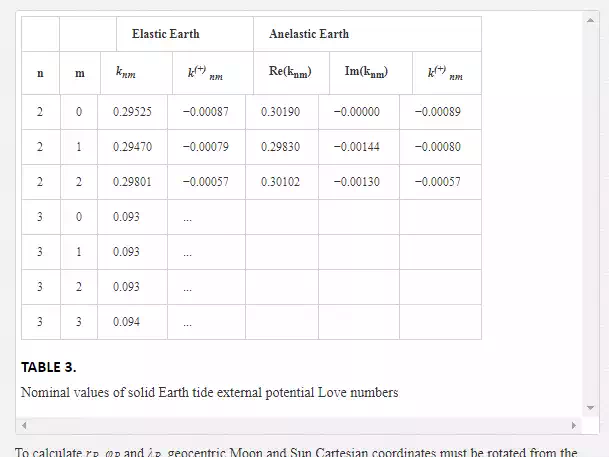
where µ* denotes the ratio of the Earth's and the Moon's masses. Since the changes induced by the Earth’s solid tides [27] due to its rotation under effects of ellipticity and Coriolis force, can be described in terms of the Love numbers, variations in the low-degree Stokes’ coefficients can be easily computed. Dependent and independent frequency corrections are calculated using lunar and solar ephemerides, Doodson’s fundamental arguments, the nominal values of the Earth’s solid tide external potential Love numbers and the in-phase and out-of-phase amplitudes of the corrections for frequency-dependent Love values. First, changes induced by the tide generating potential in the normalized geopotential coefficients for both n = 2 and n = 3 for all m are given by the frequency-independent corrections in the form:
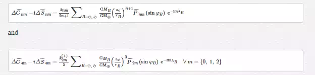
where
knm is the nominal Love number for degree n and order m,
rB is the distance from geocenter to Moon or Sun,
φB is the body-fixed geocentric latitude of Moon or Sun,
λB is the body-fixed east longitude (from Greenwich) of Moon or Sun.
Here, anelasticity of the mantle causes knm and k(+)nm to acquire small imaginary parts (Table 3).
To calculate rB, φB and λB, geocentric Moon and Sun Cartesian coordinates must be rotated from the ICRS to the ITRS and transformed to the spherical coordinates as usually.
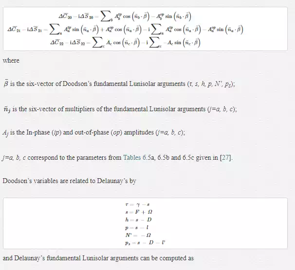
Frequency dependent corrections are computed as the sum of contributions from a number of tidal constituents belonging to the respective bands.
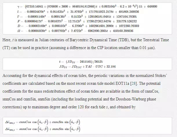
[28] also provided the influences of additional minor tide constituents that are not included in the tide model EOT11a and should not be neglected in Low Earth Orbiters. This function evaluates the contribution of altogether 256 tides.
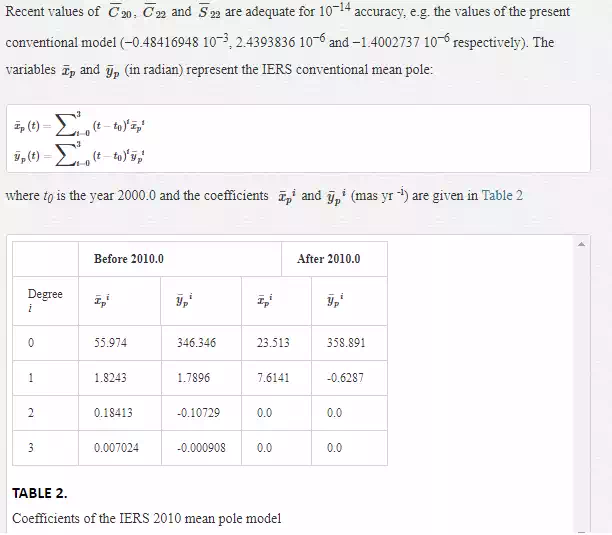
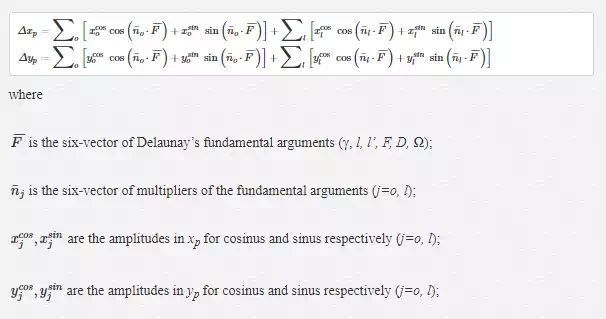
Changes in the geopotential value due to the centrifugal effect of pole motion, known as the Earth’s solid pole tides [27], can be readily computed in function of the wobble variables and calculated under sub-daily polar motion variations as
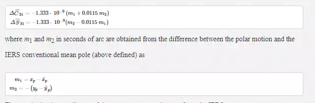
The standard pole coordinates of the parameters xp and yp are from the IERS (http://hpiers.obspm.fr/iers/eop/eopc04/) with additional components to account for the effect of ocean tides (∆xp, ∆yp)ocean and forced terms (∆xp, ∆yp)libration with periods of less than two days in space. These sub-daily variations are not part of the polar motion values published by the IERS and are therefore to be added after interpolation.
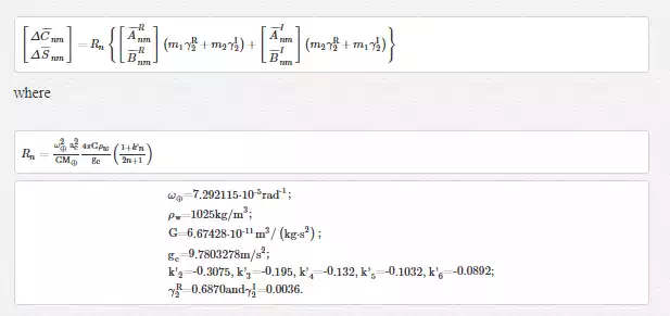
Oceanic parameters are retrieved from Tables 8.2a and 8.2b, and libration parameters (n=2) from Table 5.1a of [27]. The ocean pole tide, generated by the centrifugal effect of pole motion on the oceans, is calculated as a function of sub-daily wobble variables from the coefficients (A¯¯¯nmA¯nm and B¯¯¯nmB¯nm) of the self-consistent equilibrium model [29]. These perturbations to the normalized geopotential coefficients are given by
Only the main relativistic effects (described by the Schwarzschild field of the Earth itself ~1nm/s2), might be calculated, since the effects of the Lense-Thirring precession (frame-dragging) and the geodesic (de Sitter) precession are two orders of magnitude smaller at a near-Earth satellite orbit [27].
ACCELEROMETER CALIBRATION
The approach here given (acceleration approach) is based on the fact that the GPS-derived accelerations can provide exact values to estimate the accelerometer calibration parameters. In order to compute the differences between the GPS-based non-gravitational accelerations and the accelerometer measurements, several transformations between reference systems are required (POD solutions are usually given in the ITRS and accelerometer measurements in the SBS).
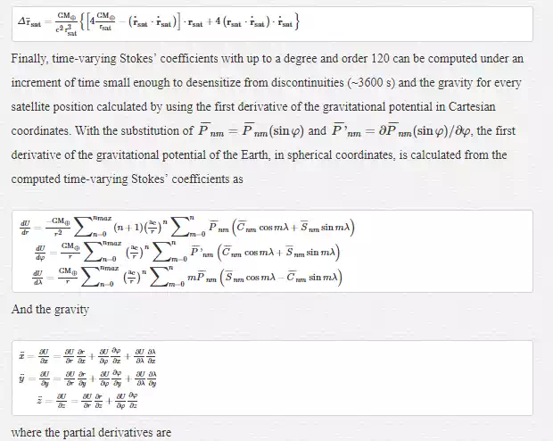
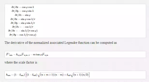
Lunisolar direct tides and the relativistic effect are calculated in the ICRS, the others, in the form of Stokes’ coefficients. The computation must be done under an increment of time small enough to desensitize from temporal variations (~3600 s). Gravitational accelerations must be rotated to the ICRS as they were positions, because the Stokes’ coefficients have already included the contribution of the Earth’s rotation. The attitude of the satellites is based on celestial body observations, so the rotation to the SBS implies to pass through the ICRS. First, the gravitational accelerations must be subtracted from the GPS-based accelerations to obtain the non-gravitational accelerations. Then, computed non-gravitational accelerations can be rotated to the SBS, and the differences to the accelerometer measurements are evaluated by means of simple difference of median averages or by Least Squares adjustment.
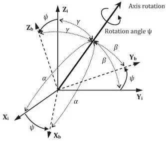
For the following, the basic rotations in the tri-axial reference system are defined as
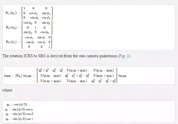
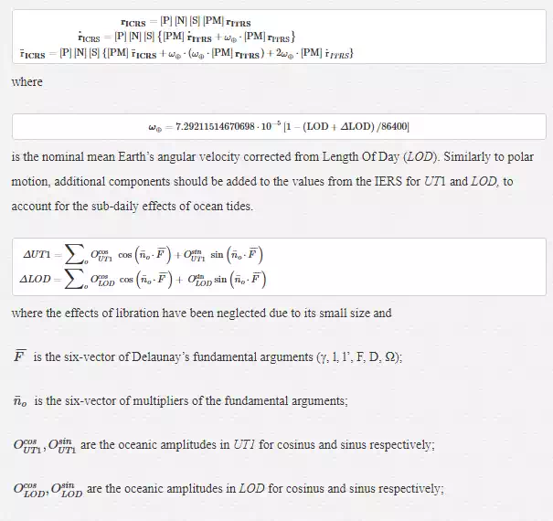
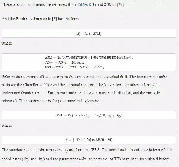
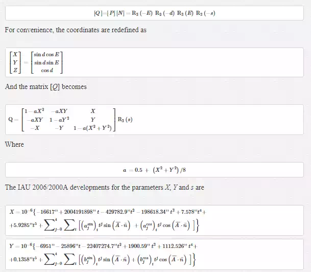
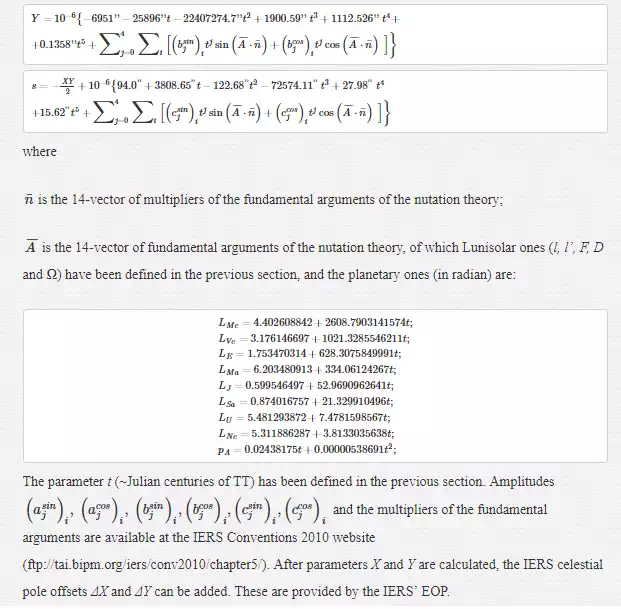
The transition from the ITRS to the ICRS is realized through a sequence of rotations that account for precession [P], nutation [N] and Earth rotation [S], including polar motion [PM] [27].
Results and analysis
GPS-BASED NON-GRAVITATIONAL ACCELERATIONS FROM GRACE
The GNI_1A files provide the most precise position and velocity at 5 s interval, including formal error (dynamic-reduced approach computed by the GPS Inferred Positioning System software of JPL). GNV_1B files are practically unchanged from the previous processing level (GNI_1A files), since only smoothing on day boundaries is applied.
Time conversion between Level 1B files and the UTC is defined as

where TFILE is the time in the Level 1 data file and UTC0 is the January 1st of 2000 at 12h 00m 00s. Since satellite accelerations are not provided in the GNV_1B files, these are derived from the precise velocities by means of interpolation and subsequent numerical differentiation. 8-data point piece-wise Lagrange interpolation is used for interpolation as recommended by [10] or [7]. In order to obtain a value to define the arc-to-chord interpolation threshold (Δt), total accelerations are calculated for several Δt and a value of Δt = 0.05 s should be chosen (error < 1nm/s2 in the arc-to-chord approximation). Then, total accelerations can be numerically obtained as the first derivative of the GNV_1B velocities.
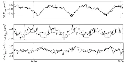
After subtracting the time-varying gravity from the GPS-based accelerations, an unknown periodic error (~1.6 hour) of amplitude maxima of ~3µm/s2 can be identified in the YSBS axis of both GRACE satellites. ZSBS axes also reveal a slightly systematic behaviour, but two orders of magnitude smaller. The underlying signal is recovered by subtracting a sinusoidal function fitted on the envelope of the modulated amplitude. Since only sinusoidal functions are removed, the resulting solution remains unchanged from mean values [10]. Figure 2 shows the results contrasted to accelerometer measurements calibrated with recommended a-priory biases of [30][30]. When analyzing the solution for XSBS axes, aside the excellent agreement with the accelerometer precision, several local mismatches can be identified and probably attributed to the non-modelled local time-varying gravity, such as post glacial rebound, hydrologic cycle, etc., due to lack of accuracy of ocean tides models or possible external sources to the Earth’s gravity, e.g. Figure 2 at 19:30 h. Concerning the YSBS and ZSBS axes solutions, aside the bias detected with respect to [30], it can be clearly seen the high correlation with the accelerometer measurements, and consequently the good reference for accelerometer calibration.
CALIBRATION OF GRACE ACCELEROMETERS
The twin satellites of the GRACE mission are equipped with three-axis capacitive SuperSTAR accelerometers to measure the non-gravitational forces. The precision of the XSBS and ZSBS axes is specified to be 0.1nm/s2, while 1nm/s2 for the YSBS axes. According to the ONERA Super Star accelerometers, the accelerations due to the relative proof mass offset and the Lorentz force can be neglected. Measurements at a second interval are included in ACC_1B files.
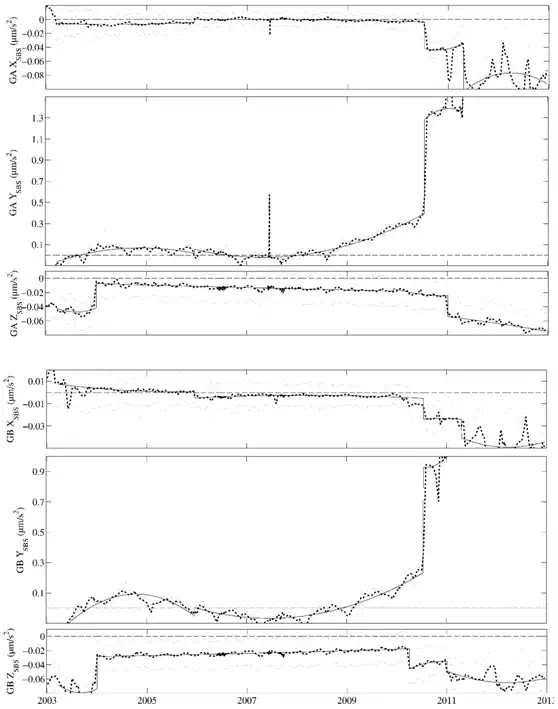
In order to evaluate the bias and bias fluctuations of the GRACE electrostatic accelerometers, the computed GPS-based non-gravitational accelerations are compared to the accelerometer measurements. Figure 3 shows the biases evaluated by simple difference of daily median averages for the 1st day and the 15th day of every month from 2003 to 2012 (240 days).
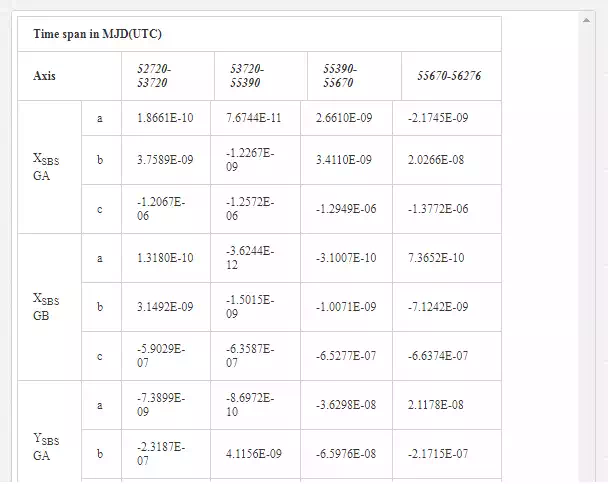
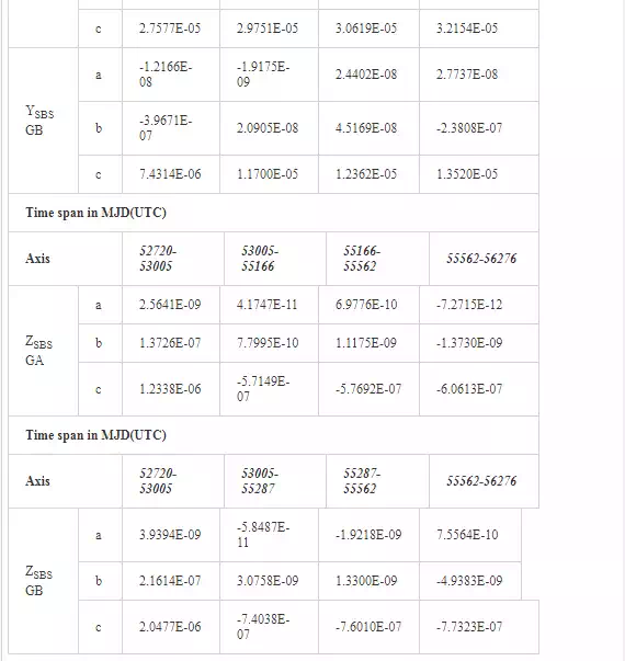
Biases and fitted approximations are plotted in Figure 3, with respect the a-priori biases as recommended by [30]. Since the nature of circular orbits implies a constant behaviour of the arc-to-chord error, the real magnitude (bigger) of radial accelerations (ZSBS axes) seems to cause a constant difference (~20 nm) in the solutions of [30]. Furthermore, it is interesting to see that since electrostatic accelerometers are sensible to temperature changes, the correlation between YSBS biases and the β’ angle (angle between the Earth-Sun line and the orbit plane) is clearly recognized. Note that the β’ angle is defined such that it is zero when the Sun is within the orbit plane and, consequently, the perturbation of YSBS biases is minimized. The opposite situation happens when maximum β’ angle, in which the solar radiation has the same direction as the YSBS axes and maximizes its bias perturbation. These variations are disregarded in the
polynomial fitting given in table 4, being this solution a more close approximation to values of β’ angle zero than the real β’ angle value.
Summary
In this chapter, a detailed theory and methodology to derive non-gravitational accelerations from GPS measurements has been review, developed and validated with GRACE satellites as an example. The results show good agreement with accelerometer measurements and demonstrate that this new approach is a good reference for accelerometer calibration. This methodology is based on the use of the arc-to-chord threshold for data interpolation, and the robust fitting of sinusoidal functions in case of finding systematic errors within the accurately derived non-gravitational accelerations.
With the development of space accelerometers, the calibration of current bias-rejection devices is not anymore required. Nevertheless, the non-gravitational accelerations can be determined accurately from the precise orbit ephemeris and, so far, it is, among others, a precious source of information for atmospheric and force model studies. With the increased accuracy of GPS positioning and dynamic measurements and models, the methodologies for GPS-based POD are becoming more and more accurate.
In order to guarantee an unbiased solution in accelerometer measurements, calibration parameters have been finally calculated without using any kind of regularization or constraint, and by using the GPS-based POD solution as a reference. Since the POD products do not use to give information about accelerations, the first derivatives of the precise-orbit velocities are calculated under the arc-to-chord interpolation-threshold. On the other hand, the modeled time-varying forces of gravitational origin and reference-system rotations are computed according to current IERS 2010 conventions (including sub-daily tide variations). In a case study from GRACE was shown that after subtracting the modeled time-varying gravity from the GPS-based accelerations, cross-track axes of both GRACE satellites are affected by a periodic error of unknown source. With the finality of extracting the underlying information from the resulting data, the systematic error is modeled and subtracted successfully by applying a robust fitting by sinusoidal functions. The resulting accelerations can serve as a reliable reference for the accelerometer calibration. In the future, this systematic error should have further considerations in POD software development.
Nomenclature
δjk; δjk; Kronecker’s delta.
ti; Instant i of time.
Δt; Increment of time.
c; Speed of light
U; Gravitational potential.
⨁; Earth.
⊙; Sun.
⊘; Moon.
GM; Product of gravitational constant by mass.
ae ; Equatorial radius of the Earth.
P¯¯¯lm; P¯lm; Normalized associated Legendre functions of degree ll and order mm.
C¯¯¯lm; C¯lm; Normalized Stokes’ coefficient of degree ll and order mm for cosinus.
S¯¯lm; S¯lm; Normalized Stokes’ coefficient of degree ll and order mm for sinus.
ω⊕; ω⊕; Rotation vector of the Earth.
r; ; Satellite position vector.
ṙ; ; Satellite velocity vector.
r¨;r¨; Satellite acceleration vector.
(φ,λ); (φ,λ); Latitude, longitude.
GPS; Global Positioning System.
POD; Precise Orbit Determination.
LEO; Low Earth Orbit
GRACE Gravity Recovery And Climate Experiment.
GA, GB; Satellite identifier (GRACE-A; GRACE-B).
EOP; Earth Orientation Parameters.
MJD; Modified Julian Date.
UTC; Coordinated Universal Time.
TAI; International Atomic Time.
ICRS; International Celestial Reference System.
ITRS; International Terrestrial Reference System.
SBS; Satellite Body System.
ORS; Orbit Reference System.
[P]; Rotation matrix for precession.
[N]; Rotation matrix for nutation.
[S]; Rotation matrix for sidereal time.
[PM]; Rotation matrix for polar motion.