Intelligent Traffic System: Implementing Road Networks with Time-Weighted Graphs

Hatem F. Halaoui¹

^[1] Haigazian University, Lebanon

Introduction

This section introduces the chapter’s main subject. First, spatial temporal and spatio-temporal databases are presented as the main databases used in all Geographical Information Systems (GISs) including driving direction systems. Second, a brief introduction of GIS is presented. Finally a brief overview of existing driving path application is included as applications similar of the work proposed here.

SPATIAL DATABASES

As most kinds of applications need databases, Geographical Information Systems use what is called spatial databases. Spatial (from space) databases are databases used to store information about geography like: geometries, positions, and coordinates. Also they include spatial operations to be applied on such kinds of data like distance, area, perimeter, direction, and overlap of geometries.

Who might use spatial databases? The following do use spatial databases:

· Mobile phone users: where is the nearest gas station?

· Army field commander: enemy movement?

· Insurance risk manager: houses to be affected?

· Medical doctor: same treatments in some area?

· Transport specialist

· Sports: what seats have good view?

· Emergency services: locate calls.

TEMPORAL AND SPATIO-TEMPORAL DATABASES

A database contains information and transactions that need to be stored, manipulated and retrieved. A number of computer applications that use databases deal only with the most recent or current data. Such a database is called snapshot databases, which represents the data at the current time with recent values. On the other hand, in some applications, users might need to know not just the current information but also past or future information as well. Databases dealing with past, present, and future data are called temporal databases or historical databases [5]. Such databases support applications such as managerial information, and geographical information. An example of this is a bank account where the customer might need to know old balances or old transactions. In such a case, users need a history of the information. These databases process a temporal dimension to store and manipulate time-varying data. In temporal databases, time is involved in two common ways [5]:

· Time stamp: one attribute is used to save the time of the validity

· Time interval: two attributes are used to indicate the interval of validity (start time and end time).

It is obvious that most spatial databases are also changing with time. For example, road networks will be constantly changing, areas of lands on maps may change, a moving plane will change its position over time, and so on. In such a case, we have spatial or geographical data that is changing with time. In this case spatial database becomes temporal as well and is called spatio-temporal database. Such databases are categorized in three main categories:

· Discretely changing spatio-temporal databases: like the changes of the geometry of land parcels where it could occur once every year or more.

· Continuously changing spatio-temporal databases: mostly deal with moving objects like plane or cars where the position of the object is changing continuously with time.

· Third category that is a combination of the above.

In reality, most spatial databases change with time and hence most of them are spatio-temporal databases.

GEOGRAPHICAL INFORMATION SYSTEMS

Geographic Information System (GIS) is a collection of computer hardware, software for capturing, managing, analyzing, and displaying all forms of geographical information [5].

Geographical Information Systems are being involved in most aspects of life and businesses. All GIS’s use spatial databases as their data warehouse that are manipulated and presented in a user interface. Later in this chapter, driving direction example queries are given as examples of GIS applications.

DRIVING PATH AND GNSS AS A GIS APPLICATIONS

Global Navigation Satellite System or GNSS is a satellite navigation system that uses satellites to provide autonomous geo-spatial positioning with global coverage. It allows small devices (especially mobile) to receive and determine their location (longitude, latitude, and altitude) to within few meters using time signals transmitted along a line-of-sight by radio waves from satellites. These devices calculate the precise time as well as position, which can be used as a reference for scientific experiments.

Finding the driving path is one of the most frequent queries in GIS applications. There are many factors that influence the criteria of finding the driving path; the following are the most important:

· Distance: What is the distance between the origin and destination?

· Road situation: is the road closed?

· Road traffic: how much traffic is on the road?

The chapter is organized as follows: this section introduces the subject in general. Section 2 presents some related and previous work including widely used applications. Section 3 presents our intelligent traffic system as the main solution of the problem at hand and finally section 4 discusses some conclusions.

Related and previous work

An overview of related practical and theoretical related work is presented in this section. Example queries are also illustrated. Moreover, the section briefly presents existing artificial intelligence in such applications. Finally, A*Traffic is presented as the main algorithm used in this chapter where a proposal of a time-weighted graph is used as the main data structure where A*Traffic is applied.

DRIVING DIRECTION APPLICATIONS: GOOGLE EARTH AS AN EXAMPLE

This sub-section presents one of the most widely used applications for finding driving directions: Google Earth. As a note, the application is not only used as driving directions application only but also offers other GIS services which are out of the scope of this chapter.

GOOGLE EARTH

Google Earth [9, 10] is a geographical system that offers satellite images of the locations along with spatial information such as coordinates and elevation. It contains about 70 TB of Data [10]. It provides three main kinds of data: Raster data, Spatial and Non-spatial data, and Video. Moreover, Google Earth offers a set of functionalities, an important subset of which is:

· Answers location queries: the user gives a location (New York, USA) as input and gets a geographical image as an output. The image can be explored in details; this feature includes: cities, businesses, public places, etc.

· Shows directions: the user gives an origin and destination as input and gets a map as output showing the directions with driving hints on the map.

· Displays spatial information: Google earth shows spatial information like coordinates, elevations, altitude, and others.

· Has learning abilities: Google Earth saves recently and regularly visited locations and queries so that the user avoids delays the next time these locations or queries asked.

· Includes pre-known locations: Google Earth offers a list of the most used locations like government offices, schools, etc.

· Provides user interaction: the user is able to put place marks on the map so he/she can avoid delays the next time visits the same place is visited.

· Provides prepaid online service that provides the customer with live video (with restriction and delay due to security) of any place in the world.

· Other products like Google Earth PRO: it is a paid service that makes it very easy to research locations and present discoveries. In just a few clicks, the user can import site plans, property lists or client sites and share the view with his/her client or colleague. Moreover, the user can export high-quality images to documents or the web.

In addition to introducing Google Earth, this section present a driving directions query as an example of the driving direction services that Google Earth offers, which is directly related to the work in this chapter.

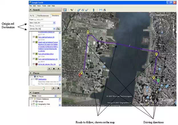
DRIVING DIRECTION QUERY BY GOOGLE EARTH: FORM “NEW YORK, NY” TO “JERSEY CITY, NJ”

Figure 1 shows the driving directions with a map image from New York, NY to Jersey City, NJ. The figure shows the input (origin and destination) and outputs on the map (Roads and driving directions). In such queries, “Google Earth” provides driving tips to be followed when driving from the origin to the destination given in the query. The user can be more specific by passing a full address (building, street, city, state, and zip assuming U.S.A. is the country.)

ARTIFICIAL INTELLIGENCE AND DRIVING DIRECTIONS

Artificial inelegance is used in graph searching algorithms. Russel and Norving [4] presents several intelligent graph searching algorithms. Here are two important ones:

· Greedy best-first search

· A* search

The main idea behind these algorithms is that they do not try all possible cases to give an answer. The algorithms use heuristic function to un-check some of the paths. This saves huge amount of time but does not guarantee a best path. However, finding a good heuristic function could guarantee up to 95% finding the best path. This section includes the A* search algorithm to be used in the solution approach presented in this chapter.

A* TRAFFIC: DESIGN, ALGORITHMS AND IMPLEMENTATION FOR A DRIVING DIRECTION SYSTEM

This section presents the application algorithms and the application of the intelligent driving path application used in our previous work, which is extended in this chapter. Examples of executions demonstrated using our testing tool, are presented.

A*: AN ARTIFICIAL INELEGANT ALGORITHM FOR FINDING DRIVING DIRECTIONS

A* [2, 4] is an Artificial Intelligent graph algorithm proposed by Pearl. The main goal of A* is to find a cheap cost graph path between two nodes in a graph using a heuristic function. The main goal of the heuristic function is to minimize the selection list at each step according to a logical and applicable criterion. In the graph example, finding the shortest path from one node to another has to be done by getting all possible paths and choosing the best. This process is very expensive and time consuming in the presence of a huge number of nodes. On the other hand, using an evaluation function (heuristic function) to minimize our choices according to intelligent and practical criterion would be much faster especially for applications requiring quick output as the driving direction application.

The heuristic function is not a constant static function. It is defined according to the problem in hand and passed to the A* as a parameter.

In the case of A* search for a direction path, the heuristic function F is built up from two main factors:

H = Straight Line distance to destination (distance between two coordinates).

G = Distance Traveled so far.

F = H + G.F = H + G.

At each node n, we compute F (n) is computed and the next step is chosen accordingly (the node with the least value of F is chosen).

THE A* ALGORITHM

A*(Origin, Destination, F)

· Define a List L that includes all visited nodes n_i with their values of F(n_i)

· Define the Stack S that includes nodes n_i with their values F(n_i)

· Start at origin (origin is the starting point)

· Mark the origin as visited

· Push origin in the stack S

· Add origin and F(origin) to L

· Get top element TE of the Stack S

· For each unmarked neighbor UN_i of TE add UN_i and F(UN_i) to L

· From L choose N: the node with the least F(N) then pop all elements in S until predecessor of N appears on the top

· Push N in the stack S

· Go back to step 5 until the destination node appears or no more unmarked nodes exist

· If no more unmarked nodes exist, return “No Solution” otherwise return the Stack content as a solution

Note that A* Algorithm is a polynomial time algorithm with time complexity in O(n²) in the worst case and O(n*logn) in the average and best cases.

Figure 2 is an example of the A* algorithm behavior to find a path starting from “Arad” to “Bucharest” in Romania [4]. First, we start at Arad and go to the next neighbor with the best heuristic function (Sibiu). Second, explore all neighbors of Sibiu for the best heuristic function (evaluation of the function is shown). The algorithm continues to choose the best next step (with the least value of heuristic function) until it reaches Bucharest.

A*TRAFFIC: A VARIATION OF A* WITH ROAD TRAFFIC AS A FACTOR

A*Traffic could be seen as a variation of A* with the ability to take traffic into consideration when computing the driving direction solution. The main job is done in the heuristic function where a new factor is used to choose the next step. The new factor is the average traffic value (got online from real time databases) represented in the following form time/distance (example: 3 min/km).

The new Heuristic function will be:

F = H + G + TF = H + G + T

Where:

H = Straight Line distance to destination (distance between two coordinates).

G = Distance Traveled so far.

T= Average Traffic delay

TESTING TOOL: QUERY EXAMPLE

This sub-section presents the layout of the testing tool developed to test the algorithm proposed “A*Traffic”. For this purpose, an example query is presented.

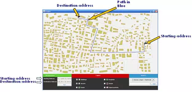
QUERY EXAMPLE: FROM “HU, KANTARI ST, HAMRA” TO “AUB, BLISS ST, HAMRA” (BEIRUT, LEBANON)

This example demonstrates the main feature of the software. It provides driving directions between “HU, Kantari St, Hamra” (Haigazian University, Beirut, Lebanon) and “AUB, Bliss St, Hamra” (American University in Beirut) in Beirut, Lebanon. In order to find the driving directions, the user has to provide a start address and a destination address and clicks on the “Go!” button. Once the button is clicked, the software generates a path (in blue) between the start and the destination addresses. The blue path generated is a short path (using A*Traffic) to follow in order to drive from the start address to the destination address. Figure 3 illustrates this example.

Road networks with time-weighted graphs

This section includes our approach in presenting the intelligent traffic system. Our main idea is to construct a time graph. We mean by the time graph: a graph representing the map with edges weighted by numbers (minutes) representing the estimated time needed to drive the edge (represent a road or part of it). The section starts by presenting the “Time-weighted Graph”, shows a possible example of the graph, gives an execution example when applying the dynamic A*Traffic algorithm proposed in our previous work.

TIME-WEIGHTED GRAPH

This section includes our graph proposal using time-weights computations possible examples and executions.

TIME WEIGHTS

Graphs are usually weighted with distances. In this chapter, time will be used as the weight of the graph edges. The main issue is: how to compute the graph edge weight in terms of time (minutes)?

To answer this question, we make the following assumptions:

· Each edge in the graph represents a road, street, highway, etc. or part of it

· Each of these (road, streets,..) has a maximum speed limit that is stored in the database

As a result:

The initial weight of the edge (minutes) = (edge distance (miles) ÷ speed (miles/hour)) * 60

EXAMPLE: PART OF MANHATTAN IN A TIME-WEIGHTED GRAPH

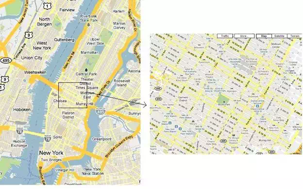
To clearly present the suggested idea, an image demonstration will be presented to show how a graph is built and weights are assigned. The following series of images show some part of Manhattan (New York, USA) in map, the process of creating vertices and edges, assigning weights for edges (using stored data) and finally applying the dynamic A* algorithm on such example. Figure 4 shows the map of Manhattan (from Google maps) and the part where the test example was done.

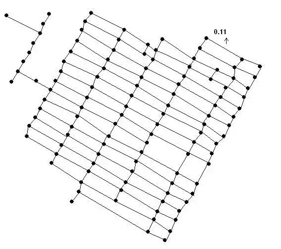
The following figures (5, 6, and 7) show the following:

· Location of vertices in the map (for simplicity, only intersection were chosen)

· Vertices only

· And finally the whole graph: vertices and edges

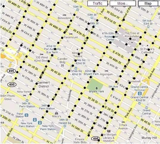
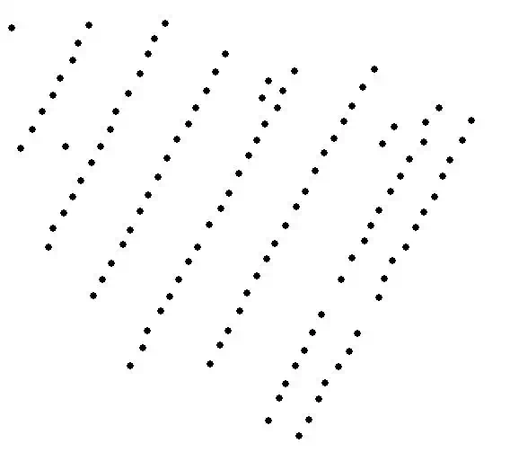
Figure 8 shows one of the edges with weight. The weight is computed as described in section 3.1.1. As a result the shown weight was computed as follows: w = 0.22 (distance) * 30 (speed) / 60 = 0.11 minutes

ONLINE UPDATES WITH DYNAMIC A*TRAFFIC

Dynamic A*Traffic assumes receiving online data whenever a related change occurs. In our new graph, the traffic system assumes receiving online data about current road situations in terms of time units. The main question is:

How can we describe the road traffic changes in time units (minutes)?

If the road is categorized as “heavy traffic”, the online system simply does the following:

· Calculates the average speed (AV) of moving vehicles (not exceeding the max limit) in the heavy traffic road

· Get the distance (D) of the road (or the part) where heavy traffic exists

· Sends T where T = (AV/D) * 60

QUERY EXAMPLE

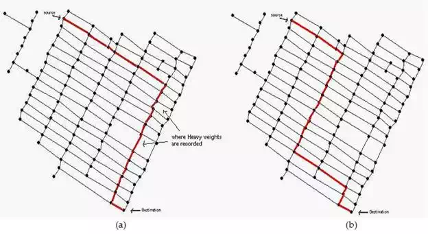
Figure 9 (a) shows a calculated query path (using A* algorithm) where figure 9 (b) shows a recalculation of the same query (with a new path) after online information about the traffic situation is received. Here are some hints of the shown calculations:

· The calculated time T1 in figure (a) is 3.35 minutes

· After receiving updated data, T1 became 5.30 minutes

· Recalculation is done and another path (figure (b))with 3.83 minutes was found

In brief, using dynamic A*Traffic algorithm and applying it on time-weighted graphs has advantages such as:

· Saves a lot of execution time when finding the path. In an optimal algorithm all possible paths have to be found and the shortest is selected among them. Such an optimal algorithm is not in P (class of polynomial time algorithms) which could take years to solve in some cases. In our case, A* and A* traffic are in P. They guarantee finding a good solution but do not guarantee an optimal solution.

· Applying time-weighted graphs takes into consideration distance and speed and as a result the algorithm will return the fastest path rather than the shortest path

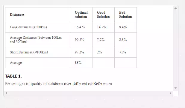
· Similar to A*Traffic, our analysis showed that our solution is optimal in 88% of the times and 97% for short driving paths. The reason for such good results is that the A* algorithm takes a lot of path related issues into consideration.

Note that our analysis now is focused on timing rather than distance and hence an optimal solution is a solution with minimum time rather than minimum distance.

Table 1 represents the results gathered from applying 100 executions in each case (long, average, and short) where:

· Optimal solution: Best solution

· Good solution: takes maximum of 30% more time than optimal solution

· Bad solution: Takes more than 30% more time than optimal solution