Stand-Alone Satellite-Based Global Positioning

Alberto Cina¹ and Marco Piras¹

^[1] Politecnico di Torino, DIATI - Department of Environment, Land and Infrastructure Engineering, Turin, Italy

Introduction

The main principle of stand-alone positioning with pseudo-range is a “multiple intersection” based on measurement of distances [1].

If the satellite’s position is known and the “range” between each satellite and the rover receiver is measured, the rover position in the same reference system of the satellite’s position could be estimated.

In this chapter, principles of measurement and least squares calculations will be discussed, with the purpose of estimating the receiver position and its accuracy. This accuracy can be “foreseen” through the DOP calculation [2], [3].

The aim of this chapter is not to show new procedures but to explain concepts described in the bibliography, often fragmentary and without examples. To improve comprehension of the values and concepts, some numeric examples are given.

Satellite positions

Each application of GPS positioning (stand-alone, relative, differential, generation of differential correction, etc) is based on knowledge of a satellite’s position in ECEF (Earth Centred Earth Fixed) geocentric cartesian reference system, which is fixed to the Earth.

The satellite position is estimated using the ephemerides which are contained in the navigation message broadcast by the satellite.

In the case of the GPS system, the ECEF satellite position is not included in this message, where dedicated parameters are contained which, following Keplerian law and considering the perturbation effect, allow calculation of the satellite position [6].

GPS ephemerides allow for the estimation of the satellite position in an inertial reference system, from which it is possible to define the ECEF coordinates.

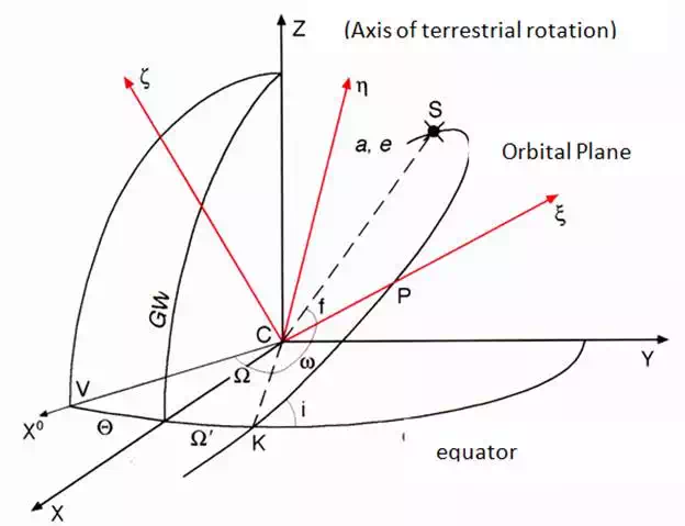
This system is described in Fig. 1 where:

V is the vernal point, the intersection of the ecliptic and the equatorial planes.

X⁰ is the axis connecting the Earth’s origin C and the point V. This direction is considered fixed, excluding some variations due to secular effects.

In the ECEF system, X is the axis of intersection of equatorial plane and the Greenwich mean meridian plane. Z is the axis which coincides with the Earth’s rotation axis and Y completes a right-handed orthogonal system.

The Greenwich meridian plane rotates around the Earth’s rotation axis with an angular speed ω_e=7.2921151467*10^-5 rad/s, in accordance with GAST (Greenwich Apparent Sideral Time).

Θ, the subtended angle between X and X⁰, is “sideral time”.

\

where:

· Ω is the longitude of the ascending node, it is the angle which has its vertex in the centre of the Earth and it is subtended by X⁰ and the ascending node K.

· P is the periapsis and it is the closest position of the satellite with respect to the Earth. The angle in C between the ascending node K and P is the periapsis argument.

· The angle i between the equatorial plane and orbital plane is the orbit inclination.

· f is the ”true anomaly”, shown in Fig. 1.

a and e² are known, the satellite position can be estimated starting from an initial position in the orbital plane, which is defined by a mean anomaly μ₀. These parameters are in the RINEX navigation message (.nav), as described in Fig. 2.

Broadcast GALILEO ephemerides are defined in the same way [10].

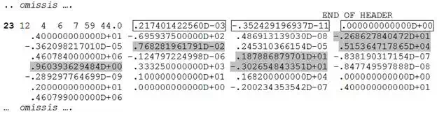
GLONASS ephemerides are instead described in a different way: navigational messages in the reference system, PZ90, already contain the ECEF position, velocity and acceleration of each satellite, estimated every 30 minutes [5].

Each set of parameters can be applied in estimating the satellite’s position 15 minutes before and after the time reference indicated in the navigation file.

A part of GLONASS navigation file is shown in Figure 3.

Satellite position is estimated using the 4^th order Runge-Kutta numerical integration of [7].

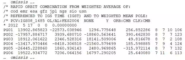
Broadcast ephemerides have about 1 meter accuracy, but more precision may be necessary for geodetic application. Precise ephemerides can be used as an alternative to broadcast ephemerides. These ephemerides are calculated “a posteriori”, and they have a centimetric level accuracy. The SP3 format [12] is used to describe these orbits and positions and satellite clock offsets are contained both for GPS and GLONASS constellations, with a rate of 15 minutes.

An example is reported in Fig. 4 [8]

Range measurement using pseudo-range

The measurement of the range between the satellite and the receiver is estimated using the pseudo-range, the code part of the signal, which is composed of squared waves. These waves are generated by an algorithm PRN (pseudo-random noise), which is periodically repeated over time [4].

In the GPS system, this component is composed of the pseudo-range C/A and P, when available. From the IIRM block, the new pseudo-range L2C is also available.

In the GLONASS system, there are two pseudo-ranges: ST (standard accuracy) and VT (usage agreed with the Russian Federation Defence Ministry) [5].

The theoretical part of the measurement of distance between the satellite and the receiver (the range) is based on the measure of “time of fly”. It is the time taken between the transmission of the signal by the satellite and the receipt by the receiver.

The range measurement is realized by means of a cross-correlation procedure between two signals. When the signal is received by the receiver, the receiver generates an identical replica and moves it with respect to time. This operation is concluded when the maximum correlation is reached (Fig. 5).

In others words, the time of fly Δt is the movement that has to be applied to the replica of the signal in order to have correct alignment with the received signal.

The two signals, received and replica, are identical, but there is a misalignment caused by the travel time in space between the satellite and the receiver, as defined in equation 1.

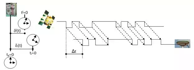
In this way, the measured distance is a “pseudo-range” because there is an offset between the satellite clock and the receiver clock.

We consider three different time reference scales (see Fig. 5):

· atomic time scale (ta), which is the GPS time fundamental reference maintained by the clocks in the control centre;

· satellite time scale (t^j), which is defined by the atomic clocks housed in each satellite;

· receiver time scale (ti), which is determined by the internal receiver clock (usually a quartz oscillator).

The satellite and receiver time scales are aligned with the fundamental scale (t_a), when the offset δ^j and δ_i are estimated. These offsets are time dependent and they have to be considered as biases in the measurement of the range.

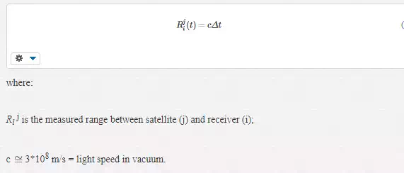
If each time is referenced to the fundamental scale, the measured range will be:

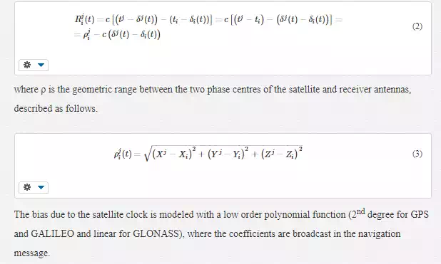
Fig. 2 and Fig. 3 give examples of the RINEX navigation files for the GPS and GLONASS constellations.

In the GPS situation, the group delay (T_GD) and the relativistic effect Δtr have to be considered, in order to estimate the satellite clock offset, using the following equation:

The velocity of a group is the velocity of the signal propagation and it is different from the single phase velocity of each component. T_GD is broadcast in the navigation message.

The relativistic effect is due to the satellite high-speed in its orbit which has to be considered in proximity to the Earth, for its mass and its potential.

The element of relativistic correction is calculated according to GPS specification [6]:

:

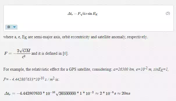
It is not possible to remove the effect of satellite clock bias in stand-alone positioning as it leads to an error of about 1 ns (10^-9 s), which corresponds to an error equal to 30 cm of the range measured between the satellite and the receiver.

The receiver clocks are typically quartz oscillators, which have less long-term stability compared to atomic clocks. On the supposition that errors of synchronization is approximately equal to 1 ms (10^-3 s). This error, in the distance between the satellite and the receiver considering speed of light, is equal to 300 km.

The receiver clock offset is difficult to model therefore an additional unknown is considered at each epoch of measurement: the bias of the receiver clock δ_i.

Separating unknown and known terms in Equation 2, the pseudo-range equation will be

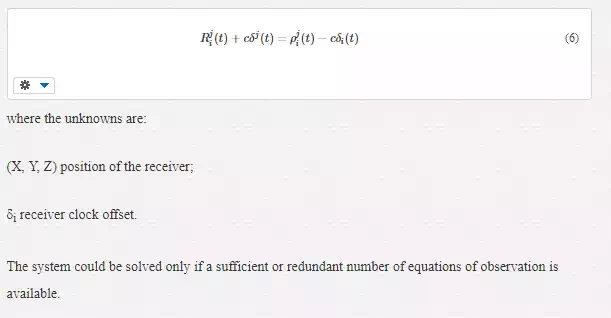
Observation equations

We consider two different types of positioning: static and kinematic.

In the first, the receiver is stationary over a point for several epochs, without changing its position. In the second, the receiver moves and its coordinates change in each epoch. In the kinematic, four unknowns have to be solved for each epoch: three for the position (X, Y, Z) and one for the receiver clock offset [9].

Linearization of Equation (6) and considering the approximate values of the receiver position, as:

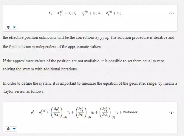
It is convenient to define the offset of the receiver clock in metres, in order to avoid possible problems of ill conditioning of the system, due to the light speed c which is prevalent with respect to the other values. This is easily achievable, multiplying the offset by the light speed.

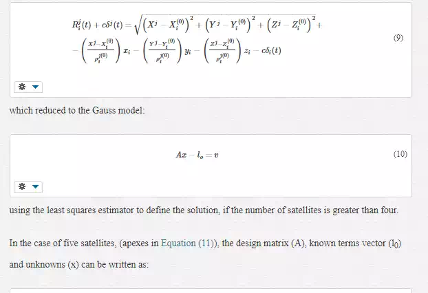
This positioning model with pseudo-range measurement defines a single position at each epoch and is useful for kinematic procedures.

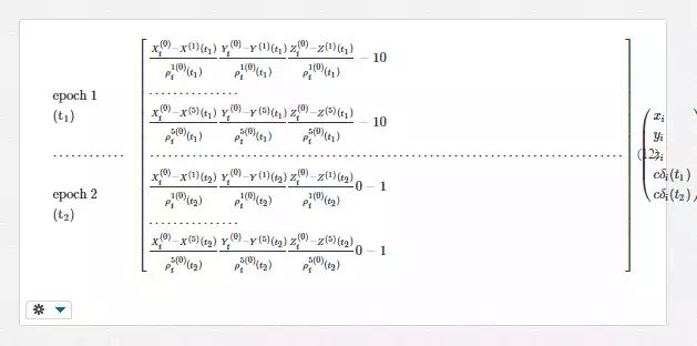
The static solution requires adding additional columns in the design matrix (A), in order to estimate the offset of the receiver clock at each epoch.

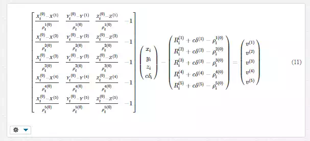
To consider 2 epochs of measurement in static session, Equation (11) has to be modified as follows:

Least Squares

The least squares solution starts from the Gauss model, which was described in (10), and is defined by means of calculus and inversion of the normal matrix N.

The estimated residuals 

vˆv^

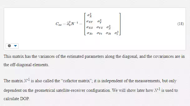
 and the variance–covariance matrix of the estimated solution C_xx can be calculated, considering:

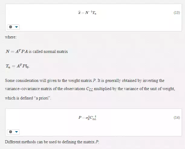
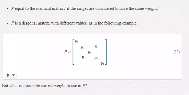
There are different strategies used to selecting the weight of the range:

· Starting from the URA (User Range Accuracy), which represents the maximum error of the range foreseen during the period of validation of the ephemerides, it is a statistical value of the accuracy for each satellite. URA is contained in the navigation message and it is independent of the satellite’s elevation or other environmental conditions. Using the GPS specification the accuracy of each satellite can be estimated [13].

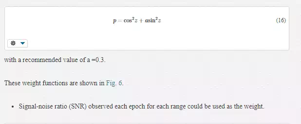
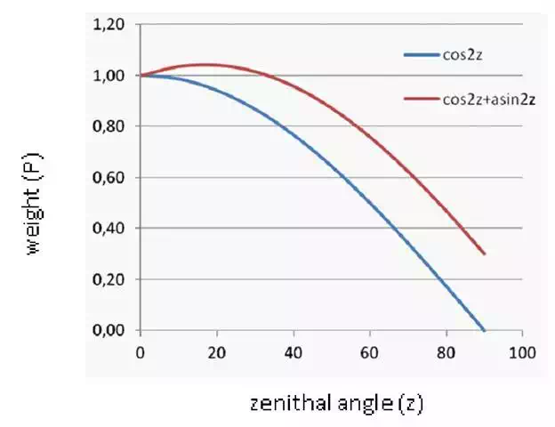
· Each weight can be considered depending on the satellite’s elevation. For example, a function of the zenithal angle z can be used, where each satellite can be weighted with the following model: 

p=cos2zp=cos2z

. EUREF suggests an alternative method [11]:

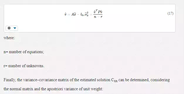
Based on the estimated solution 

xˆx^

, the estimated residuals 

vˆv^

, and the apostriori variance of the unit weight, can be obtained:

Measurement bias of the pseudo-range

In order to consider the several range measurement biases, Equation (6) has to be modified as follows:

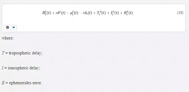
A short description will be given in the following.

Tropospheric delay is an error which occurs in only the low part of the atmosphere, up to 40 km from the Earth’s surface.

This error depends on: pressure, temperature and relative humidity. It can be estimated using a model, such as the one described in [3, 4]. In the standard condition (i.e. temperature =273.16 K, pression=1013.25 mbar, e=0), this error is equal to 2.3 m in the zenith position (z=0°) and it increases when the zenithal angle increases.

This is the main reason that it is better to avoid using satellites with low elevation (zenithal angle > 75°) to realize the positioning.

Ionospheric delay, on the other hand, depends on the electronic content of the ionosphere layer of the atmosphere between 40 km and 1000 km above the Earth’s surface; it changes with the sun’s activities. This delay is dispersive, that is, it depends on the signal frequency. The value of this delay is variable but it is normally greater than the tropospheric delay. Dual frequencies receivers can use the dispersive nature of the ionosphere to completely remove the delay.

Ephemeride errors depend on the satellite position: broadcast ephemerides have a meter-level accuracy; precise or predicted rapid products instead have centimeter level of accuracy. These products are available on the IGS (International GNSS Service) website.

These errors are spatially correlated; therefore they have similar effects on two receivers in close proximity. These biases can be eliminated or reduced using relative positioning, but not in the stand-alone positioning.

Others errors such as phase centre variation, multipath and hardware delay are less significant in this context and are not considered.

Relative motion in the stand-alone positioning

The position, estimated as described above, does not consider certain important effects which happen during the time of the propagation of the signal from the satellite to the receiver (about 67 ms).

The following effects occur during this period:

· the satellite position is changed by about 250 m;

· the Earth has rotated about its spin axis by about 30 m to the East on the equator.

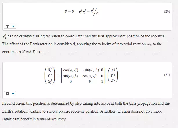
The estimation of the receiver position requires an additional iteration where the satellite position is modified, taking into account the propagation time τ.

DOP and satellite visibility

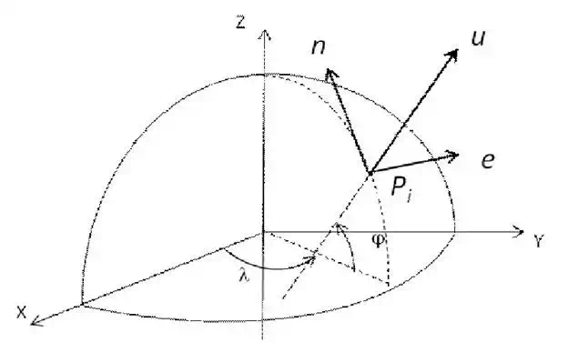
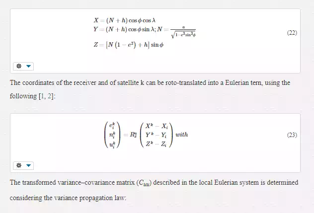
Sometimes it could be useful to define the ECEF coordinates with respect to a local plane, which is tangential to the ellipsoid at a defined point. This local system allows the separation of the horizontal component from the vertical, where the GPS is less precise. If this system is used, the variance–covariance matrix has also to be rotated.

Therefore, it is possible to define a local plane with its origin at P_i, with geographical coordinates φ and λ, considering an Eulerian Cartesian tern, defined as following:

· u-axis coincides with the normal to the ellipsoid passing through P_i;

· n-axis coincides with the meridian tangent directed north;

· e-axis completes the clockwise tern.

This operation called “planning”, only requires knowing the receiver position and the almanac of the ephemerides used to determine the satellite’s position. DOPs are like an instantaneous picture of the constellation. High values (for example GDOP > 6) are inadvisable to reach a good precision.

Azimuth A, elevation E and distance d of the different satellites can be estimated in order to plan the measurement session. Each element is determined by the following equations:

Appendix A

DOP AND SATELLITE VISIBILITY       

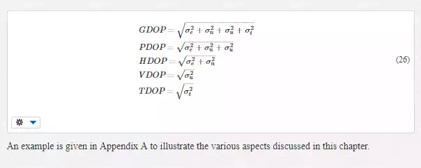
Estimate GDOP, PDOP, HDOP, VDOP, TDOP factors at P with coordinates: φ=45°3’48”, λ=7°39’41”, h=0 m, referenced in WGS84 (a=6378137 e2=0.006694379990) ellipsoid, on 2012/04/06 at 8:53:59 am. Moreover Calculate the “satellite visibility” at P. The ECEF coordinates of the visible satellites are known [8]:

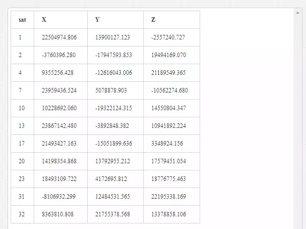
In the following, the solution is provided.

The geographical coordinates are transformed to a DEG system:

E=atnujnj2+ej2√A=atnejnkd=ej2+nj2+uj2−−−−−−−−−−−√E=atnujnj2+ej2A=atnejnkd=ej2+nj2+uj2

from which the geocentric coordinates of P are obtained.

φ=45.07333333°              λ=7.791388889°φ=45.07333333°              λ=7.791388889°

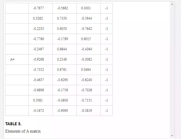
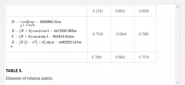
P will be the origin of the Eulerian local system. A matrix is calculated in the ECEF system considering (11), with the following values:

From which the cofactor matrix as (13) and (18) are obtainable using the weight matrix equal to the identity (P=I)

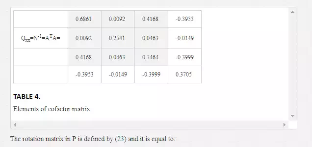
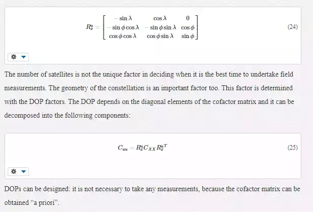
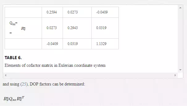
The cofactor matrix is now calculated in a Eulerian coordinate system considering (24), applying this equation only to the position components (grey elements in the Qxx matrix) and not to the time element:

Nomenclature

DOP = Dilution of precision

ECEF = Earth Centred Earth Fixed

GLONASS= Globalnaya Navigatsionnaya Sputnikovaya Sistema

GNSS = Global Navigation Satellite Systems

GPS = Global Positioning System

RINEX = Receiver Independent Exchange Format

URA = User Range Accuracy