Dimensional Analysis: From Atomic Bombs to Wind Tunnel Testing

Despite the growing computer power and increasing sophistication of computational models, any design meant operate in the real world requires some form of experimental validation. The idealist modeller, me included, wants to believe that computer simulation will replace all forms of experimental testing and thereby allow for much faster design cycles. The issue with this is that random imperfections, and most importantly their concurrence, are very hard to account for robustly, especially when operating in nonlinear domains. As a result, the quantity and quality of both computational and experimental validation have increased in lockstep over the few last decades.

In “The Wind and Beyond”, the autobiography of Theodore von Kármán, one of the pre-eminent aerospace engineers and scientists of the 20th century, von Kármán recounts a telling episode regarding the role of wind tunnel testing in the development of the Douglas DC-3, the first American commercial jetliner. Early versions of the DC-3 faced a problem with aerodynamic instabilities that could throw the airplane out of control. A similar problem had been noticed earlier on the Northrop Alpha airplane, which, like the DC-3, featured a wing that was attached to the underside of the fuselage. When two of von Kármán’s assistants, Major Klein and Clark Millikan, subjected a model of the Alpha to high winds in a wind tunnel, the model aircraft started to sway and shake violently. In the following investigation, Klein and Millikan found that the sharp corner at the connection between the wing and fuselage decelerated the air as it flowed past, causing boundary layer separation and a wake of eddies. As these eddies broke away from the trailing edge of the wing, they adversely impacted the flow over the horizontal stabiliser and vertical tail fin at the rear of the aircraft and resulted in uncontrollable vibrations.

Northrop Alpha (Y1C-19)

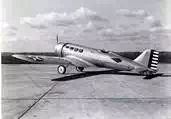
The Northrop Alpha plane with the Kármán fillet at the wing-fuselage joint

Fortunately, Theodore von Kármán was world-renowned, among other things, for his work on eddies and especially the so-called von Kármán Vortex Street. Von Kármán therefore intuitively realised what had to be done to eliminate the creation of these eddies. Von Kármán and his colleagues fitted a small fairing, a filling if you like, to the connection between the wing and the fuselage to smooth out the eddies. This became one of the textbook examples of how wind tunnel findings could be applied in a practical way to iron out problems with an aircraft. When French engineers learned of the device from von Kármán at a conference a few years later, they were so enamoured that such a simple idea could solve such a big problem that they named the fillet a “Kármán”.

When testing the aerodynamics of aircraft, the wind tunnel is indispensable. The Wright brothers built their own wind tunnel to validate the research data on airfoils that had been recorded throughout the 19th century. One of the most important pieces of equipment in the early days of NACA (now NASA) was a variable-density wind tunnel, which by pressurising the air, allowed realistic operating conditions to be simulated on 1/20th geometrically-scaled models.

Variable Density Tunnel - GPN-2000-001311

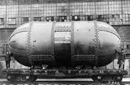
NACA variable density wind tunnel

This brings us to an important point: How do you test the aerodynamics of an aircraft in a wind-tunnel?

Do you need to build individual wind-tunnels big enough to fit a particular aircraft? Or can you use a smaller multi-purpose wind tunnel to test small-scale models of the actual aircraft? If this is the case, how representative is the collected data of the actual flying aircraft?

Luckily we can make use of some clever mathematics, known as dimensional analysis, to make our life a little easier. The key idea behind dimensional analysis is to define a set of dimensionless parameters that govern the physical behaviour of the phenomenon being studied, purely by identifying the fundamental dimensions (time, length and mass in aerodynamics) that are at play. This is best illustrated by an example.

The United States developed the atomic bomb during WWII under the greatest security precautions. Even many years after the first test of 1945 in the desert of New Mexico, the total amount of energy released during the explosion remained unknown. The British scientist G.I. Taylor then famously estimated the total amount of energy released by the explosion simply by using available pictures showing the explosion plume at different time stamps after detonation.

Nuclear Explosion Time Frames

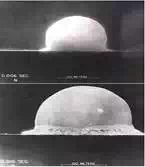
Nuclear explosion time frames

By assuming that the shock wave could be modelled as a perfect sphere, Taylor posited that the size of the plume, i.e. the radius , should depend on the energy of the explosion, the time after detonation and the density $Title: \rho - Description: \rho$ of the surrounding air.

In dimensional analysis we proceed to define the fundamental units or dimensions that quantify our variables. So in this case:

● Radius is defined by a distance, and therefore the units are length, i.e.

● The units of time are, you guessed it, time, i.e.

● Energy is force times distance, where a force is mass times acceleration, and acceleration is distance divided by time squared i.e. $Title: [E] = \left(\frac{ML}{T^2}\right)L = \frac{M L^2}{T^2}. - Description: [E] = \left(\frac{ML}{T^2}\right)L = \frac{M L^2}{T^2}.$

● Density is mass divided by volume, where volume is a distance cubed, i.e. $Title: [\rho] = \frac{M}{L^3}. - Description: [\rho] = \frac{M}{L^3}.$

Having determined all our variables in the fundamental dimensions of distance, time and mass, we now attempt to relate the radius of the explosion to the energy, density and time. If we assume that the radius is proportional to these three variables, then dividing the radius by the product of the other three variables must result in a dimensionless number. Hence,

$Title: c = \frac{R}{E^x \rho^y t^z} - Description: c = \frac{R}{E^x \rho^y t^z}$

Or alternatively, all fundamental dimensions in the above fraction must cancel:

$Title: \frac{L}{\left(M L^2 / T^2\right)^x \left(M / L^3\right)^y T^z} = \frac{L}{M^{\left(x+y\right)} L^{\left(2x-3y\right)} T^{\left(-2x+z\right)}} = M^{\left(-x-y\right)} L^{\left(1-2x+3y\right)} T^{\left(2x-z\right)} - Description: \frac{L}{\left(M L^2 / T^2\right)^x \left(M / L^3\right)^y T^z} = \frac{L}{M^{\left(x+y\right)} L^{\left(2x-3y\right)} T^{\left(-2x+z\right)}} = M^{\left(-x-y\right)} L^{\left(1-2x+3y\right)} T^{\left(2x-z\right)}$

For all units to disappear we need:

$Title: -x-y = 0 \qquad 1-2x+3y=0 \qquad 2x - z =0 - Description: -x-y = 0 \qquad 1-2x+3y=0 \qquad 2x - z =0$

and solving this system gives:

$Title: x = 1/5 \qquad y = -1/5 \qquad z = 2/5 - Description: x = 1/5 \qquad y = -1/5 \qquad z = 2/5$

Therefore the shock wave radius is given by

$Title: R = c E^{1/5} \rho^{-1/5} t^{2/5} - Description: R = c E^{1/5} \rho^{-1/5} t^{2/5}$

and by re-arranging

$Title: E = k \frac{R^5 \rho}{t^2} - Description: E = k \frac{R^5 \rho}{t^2}$

where $Title: k = \frac{1}{c^5} - Description: k = \frac{1}{c^5}$ .

So, we have an expression that relates the energy of the explosion to the radius, the density of air and time after detonation, which were all available to Taylor from the individual time stamps (these provided a diameter estimate and the time after detonation. The density of the air was known).

In the example above, specific calculations of also require an estimate of the constant . In aerodynamics, we are typically interested in quantifying the constant itself using the variables at hand. Hence, by analogy with the above example, we would know the energy, the density, radius and time and then calculate a value for the constant under these conditions. As the constant is dimensionless, it allows us to make an unbiased judgement of the flow conditions for entirely different and unrelated problems.

The most famous dimensionless number in aerodynamics is probably the Reynolds number which quantifies the nature of the flow, i.e. is it laminar (nice and orderly in layers that do not mix), or is it turbulent, or somewhere in between?

In determining aerodynamic forces, two of the important variables we want to understand and quantify are the lift and drag. Particularly, we want to determine how the lift and drag vary with independent parameters such as the flight velocity, wing area and the properties of the surrounding area.

Using a similar method as above, it can be shown that the two primary dimensionless variables are the lift () and drag coefficients (), which are defined in terms of lift (), drag (), flight velocity (), static fluid density ( $Title: \rho - Description: \rho$ ) and wing area ().

Lift coefficient:

$Title: C_L = \frac{L}{1/2 \rho U^2 S} - Description: C_L = \frac{L}{1/2 \rho U^2 S}$

Drag coefficient:

$Title: C_D = \frac{D}{1/2 \rho U^2 S} - Description: C_D = \frac{D}{1/2 \rho U^2 S}$

where $Title: 1/2 \rho U^2 - Description: 1/2 \rho U^2$ is known as the dynamic pressure of a fluid in motion. When the dynamic pressure is multiplied by the wing area, , we are left with units of force which cancel the unit of lift () and drag (), thus making and dimensionless.

As long as the geometry of our vehicle remains the same (scaling up and down at constant ratio of relative dimensions, e.g. length, width, height, wing span, chord etc.), these two parameters are only dependent on two other dimensionless variables: the Reynolds number

$Title: Re = \frac{\rho U c}{\mu} - Description: Re = \frac{\rho U c}{\mu}$

where and are characteristic flow velocity and length (usually aerofoil chord or wingspan), and the the Mach Number

$Title: M = \frac{U}{U_{sound}} = \frac{U}{\sqrt{\gamma R T}} - Description: M = \frac{U}{U_{sound}} = \frac{U}{\sqrt{\gamma R T}}$

which is the ratio of aircraft speed to the local speed of sound.

Let’s recap what we have developed until now. We have two dimensionless parameters, the lift and drag coefficients, which measure the amount of lift and drag an airfoil or flight vehicle creates normalised by the conditions of the surrounding fluid ( $Title: 1/2 \rho U^2 - Description: 1/2 \rho U^2$ ) and the geometry of the lifting surface (). Hence, these dimensionless parameters allow us to make a fair comparison of the performance of different airfoils regardless of their size. Comparing the and of two different airfoils requires that the operating conditions be comparable. They do not have to be exactly the same in terms of air speed, density and temperature but their dimensionless quantities, namely the Mach number and Reynolds number, need to be equal.

As an example consider a prototype aircraft flying at altitude and a scaled version of the same aircraft in a wind tunnel. The model and prototype aircraft have the same geometrical shape and only vary in terms of their absolute dimensions and the operating conditions. If the values of Reynolds number and Mach number of the flow are the same for both, then the flows are called dynamically similar, and as the geometry of the two aircraft are scaled version of each other, it follows that the lift and drag coefficients must be the same too. This concept of dynamic similarity is crucial for wind-tunnel experiments as it allows engineers to create small-scale models of full-sized aircraft and reliably predict their aerodynamic qualities in a wind tunnel.

This of course means that the wind tunnel needs to be operated at entirely different temperatures and pressures than the operating conditions at altitude. As long as the dimensions of the model remain in proportion upon scaling up or down, the model wing area scales with the square of the wing chord, i.e. is proportional to . We know from the explanation above that for a certain combination of Mach number and Reynolds number the lift and drag coefficients are fixed.

Using the definition of and the lift is given by

$Title: L = C_L * (1/2 \rho U^2 S) - Description: L = C_L * (1/2 \rho U^2 S)$

and the drag by

$Title: D = C_D * (1/2 \rho U^2 S) - Description: D = C_D * (1/2 \rho U^2 S)$

The lift and drag created by an aircraft or model under constant Mach number and Reynolds number scale with the wing area or the wing chord squared. Rearranging the equation for the Reynolds number, the wing chord can in fact be shown to be proportional to the operating temperature and pressure of the fluid flow. So by rearranging the Reynolds number equation:

$Title: Re = \frac{\rho U c}{\mu} \Rightarrow c = \frac{Re \mu}{\rho U} - Description: Re = \frac{\rho U c}{\mu} \Rightarrow c = \frac{Re \mu}{\rho U}$

and from the fundamental gas equation

$Title: \rho = \frac{P}{RT} - Description: \rho = \frac{P}{RT}$

and the Mach Number we have

$Title: U = M \sqrt{\gamma RT} - Description: U = M \sqrt{\gamma RT}$

such that we can reformulate the chord length as follows

$Title: c = \frac{Re \mu RT}{P M \sqrt{\gamma RT}} = \frac{Re \mu \sqrt{RT}}{P M \sqrt{\gamma}} - Description: c = \frac{Re \mu RT}{P M \sqrt{\gamma RT}} = \frac{Re \mu \sqrt{RT}}{P M \sqrt{\gamma}}$

Hence, the chord of the model is inversely proportional to the fluid pressure and directly proportional to the square of the fluid temperature. Thus, maximising the pressure and reducing the temperature (maximum fluid density) reduces the required size of the model and the overall aerodynamic forces. The was the concept behind NACA’s early variable density tunnel and is still exploited in modern cryogenic wind tunnels.