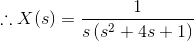
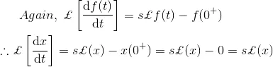
The time function f(t) is obtained back from the Laplace transform by a process called inverse Laplace transformation and denoted by £-1

Method of Laplace Transform
The Laplace transformation is an important part of control system engineering. To study or analyze a control system, we have to carry out the Laplace transform of the different functions (function of time). Inverse Laplace is also an essential tool in finding out the function f(t) from its Laplace form. Both inverse Laplace and Laplace transforms have certain properties in analyzing dynamic control systems. Laplace transforms have several properties for linear systems. The different properties are:
Linearity, Differentiation, integration, multiplication, frequency shifting, time scaling, time shifting, convolution, conjugation, periodic function. There are two very important theorems associated with control systems. These are :
The Laplace transform is performed on a number of functions, which are – impulse, unit impulse, step, unit step, shifted unit step, ramp, exponential decay, sine, cosine, hyperbolic sine, hyperbolic cosine, natural logarithm, Bessel function. But the greatest advantage of applying the Laplace transform is solving higher order differential equations easily by converting into algebraic equations.
There are certain steps which need to be followed in order to do a Laplace transform of a time function. In order to transform a given function of time f(t) into its corresponding Laplace transform, we have to follow the following steps:
The time function f(t) is obtained back from the Laplace transform by a process called inverse Laplace transformation and denoted by £-1
The main properties of Laplace Transform can be summarized as follows:
Linearity: Let C1, C2 be constants. f(t), g(t) be the functions of time, t, then
First shifting Theorem:
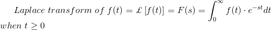
Change of scale property: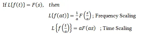
Differentiation: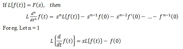
Integration: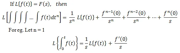
Time Shifting:
If L{f(t) } = F(s), then the Laplace Transform of f(t) after the delay of time, T is equal to the product of Laplace Transform of f(t) and e-st that is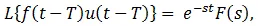
Where, u(t-T) denotes unit step function.
Product:
If L{f(t) }=F(s), then the product of two functions, f1 (t) and f2 (t) is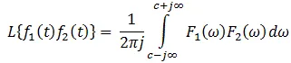
Final Value Theorem:
This theorem is applicable in the analysis and design of feedback control system, as Laplace Transform gives solution at initial conditions
Initial Value Theorem:
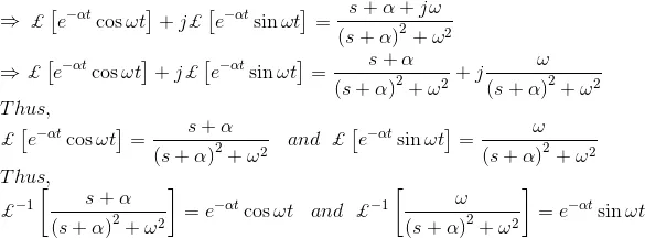
Let us examine the Laplace transformation methods of a simple function f(t) = eαt for better understanding the matter.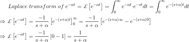
Comparing the above solution, we can write,
Similarly, by putting α = 0, we get,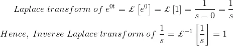
Similarly, by putting α = jω, we get,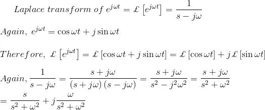

And thus,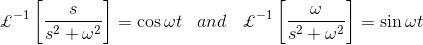
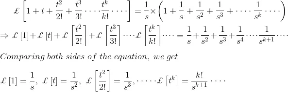
Let us examine another example of Laplace transformation methods for the function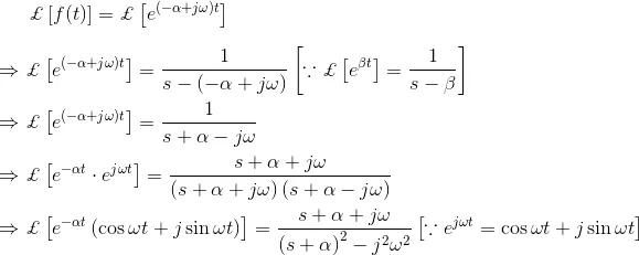
Again the Laplace transformation form of et is,
This Laplace form can be rewritten as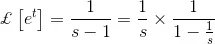
Now from the definition of power series we get,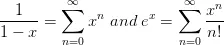
Solve the equation using Laplace Transforms,
Using the table above, the equation can be converted into Laplace form:
Using the data that has been given in the question the Laplace form can be simplified.
Dividing by (s2 + 3s + 2) gives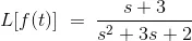
This can be solved using partial fractions, which is easier than solving it in its previous form. Firstly, the denominator needs to be factorized.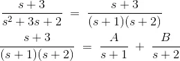
Cross-multiplying gives:
Next the coefficients A and B need to be found
Substituting in the equation: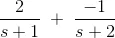
Then using the table that was provided above, that equation can be converted back into normal form.
Examples to try yourself
Calculate and write out the inverse Laplace transformation of the following, it is recommended to find a table with the Laplace conversions online: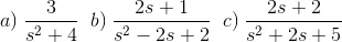
Solutions: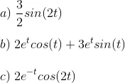
Let’s dig in a bit more into some worked laplace transform examples:
1) Where, F(s) is the Laplace form of a time domain function f(t). Find the expiration of f(t).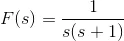
Solution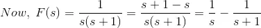
Now, Inverse Laplace Transformation of F(s), is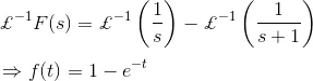
2) Find Inverse Laplace Transformation function of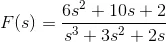
Solution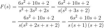
Now,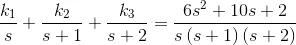

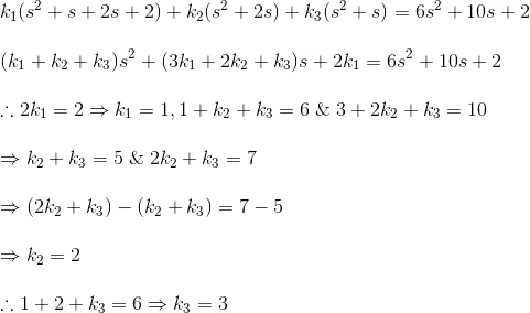
Hence,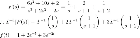
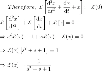
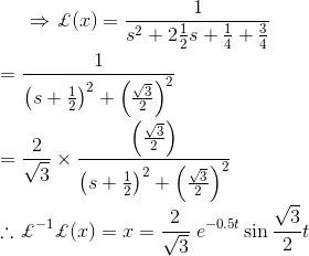
3) Solve the differential equation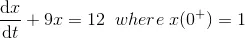
Solution
As we know that, Laplace transformation of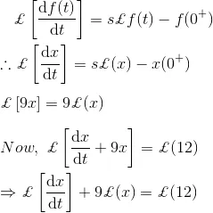
4) Solve the differential equation,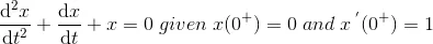
Solution
As we know that,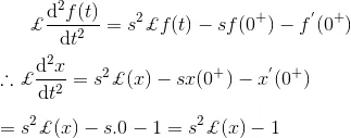
5) For circuit below, calculate the initial charging current of capacitor using Laplace Transform technique.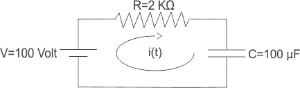
Solution
The above figure can be redrawn in Laplace form,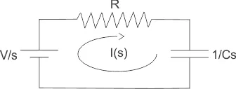
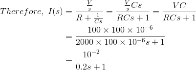
Now, initial charging current,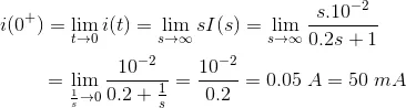
6) Solve the electric circuit by using Laplace transformation for final steady-state current
Solution
The above circuit can be analyzed by using Kirchhoff Voltage Law and then we get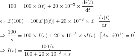
Final value of steady-state current is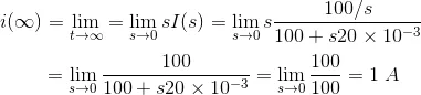
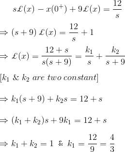
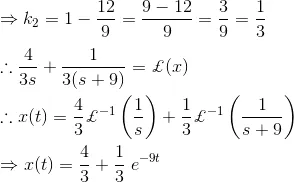
7) A system is represented by the relation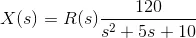
Where, R(s) is the Laplace form of unit step function. Find the value of x(t) at t → ∞.
As R(s) is the Laplace form of unit step function, it can be written as
Solution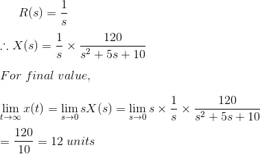
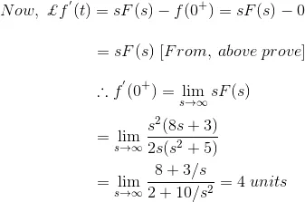
8) Find f(t), f‘(t) and f“(t) for a time domain function f(t). The Laplace Transformation form of the function is given as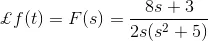
By applying initial value theorem, we get,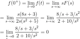
Applying Initial Value Theorem, we get,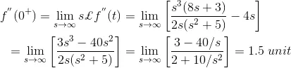
9) The Laplace Transform of f(t) is given by,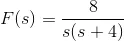
Find the final value of the equation using final value theorem as well as the conventional method of finding the final value.
Solution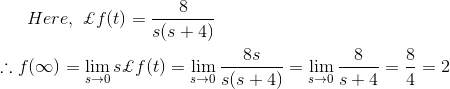
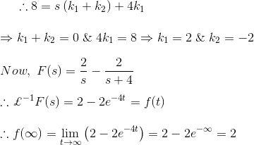
Hence it is proved that from both of the methods the final value of the function becomes same.
10) Find the Inverse Laplace Transformation of function,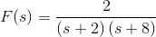
Solution
F(s) can be rewritten as,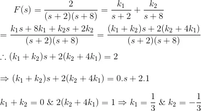

11) Find the Inverse Laplace transformation of
Solution
F(s) can be rewritten as,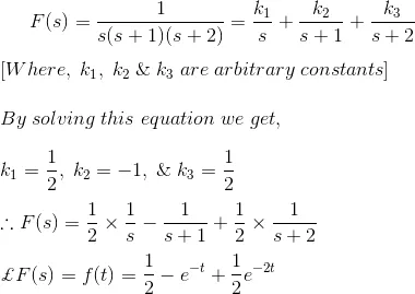
12) Find the Inverse Laplace transformation of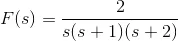
Solution
F(s) can be rewritten as,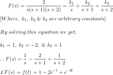
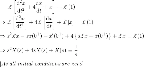
13) Express the differential equation in Laplace transformation form
Solution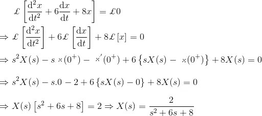
14) Express the differential equation in Laplace transformation form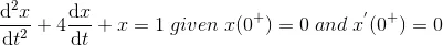
Solution