Inertial Sensors
Inertial sensors are sensors based on inertia and relevant measuring principles. These range from Micro Electro Mechanical Systems (MEMS) inertial sensors, measuring only few mm, up to ring laser gyroscopes that are high-precision devices with a size of up to 50cm. Within this note, we will briefly summarize these cases of inertial sensors that are most important to the autonomous navigation of unmanned aircraft. Inertial sensors for aerial robotics typically come in the form of an Inertial Measurement Unit (IMU) which consists of accelerometers, gyroscopes and sometimes also magnetometers. Subsequently, we will briefly summarize the main principles of accelerometers and gyroscopes widely used in unmanned aviation.
Accelerometers
Accelerometers are devices that measure proper acceleration ("g-force"). Proper acceleration is not the same as coordinate acceleration (rate of change of velocity). For example, an accelerometer at rest on the surface of the Earth will measure an acceleration g= 9.81 m/s^2 straight upwards. By contrast, accelerometers in free fall orbiting and accelerating due to the gravity of Earth will measure zero.
Accelerometers are electromechanical devices that are able of measuring static and/or dynamic forces of acceleration. Static forces include gravity, while dynamic forces can include vibrations and movement. Accelerometers can measure acceleration on 1, 2 or 3 axes. Currently, 3-axes devices are becoming more common due to the great cost reduction. Figure 1 depicts the axes found on such a device. It is highlighted that the accelerometer will measure according to its own body of reference and based on the effect of the external forces on it.
| 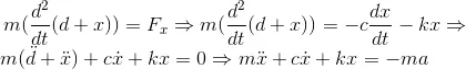
Figure 1: Axes of a 3-axes accelerometer. |
A simplified accelerometer model is depicted in Figure 2. It consists of the mass (m), the spring-damper system (k,c), the transducer and the overall component is rigidly attached on a vehicle. The displacement of the vehicle from an inertially fixed point is denoted as d, while the displacement of the test mass m from its rest point is denoted as x. Therefore:
| 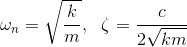
Figure 2: Simplified model of an accelerometer. |
where α is the acceleration (second derivative of d). This essentially is a second order Linear Time Invariant (LTI) model. It has the vehicle real acceleration as an input and its output is the negative of indicated test mass displacement times k/m. Its block diagram is shown on Figure 3.

Figure 3: Block diagram of the simplified accelerometer model.
Note that for the cases within which, the vehicle acceleration is constant, then the steady state output of the accelerometer is also constant, therefore indicating the existence and value of the acceleration. Finally, as shown from the second order ODE above, the undamped natural frequency and the damping ratio of the accelerometer are:
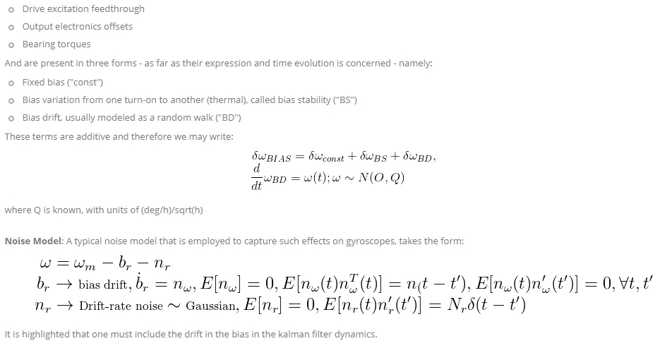
Bias effects on accelerometers: accelerometer measurements are degradated by scale errors and bias effects. A typical error model takes the form:

where a3D stands for the 3-axes acceleration vector, Macc for combined scale factor and misalignment compensation, a3D^m for the measurement and abias for the measurement bias.
References and further readings:
- "Dynamics" course MIT OCW, Instructors: Prof. Sheila Widnall, Prof. John Deyst, Prof. Edward Greitzer, http://ocw.mit.edu/courses/aeronautics-and-astronautics/16-07-dynamics-fall-2009/
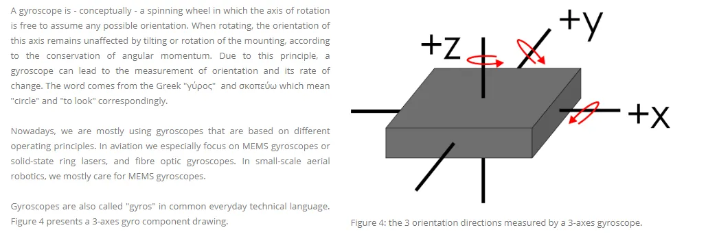
Gyroscopes